
Isolating Structural Parameter Drift From Transient Environmental Noise In Dynamic Calibration Analysis
Dynamic calibration isolates structural parameter drift from transient environmental noise through timescale decoupling and statistical innovation tests.
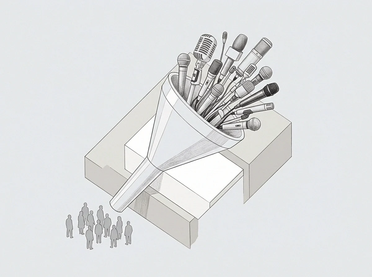
Bench
Dynamic calibration routines run continuously inside systems exposed to fluctuating operating regimes. Physical degradation changes structural stiffness, mechanical friction, and sensor zero-points over prolonged periods. Ambient temperature shifts, atmospheric gusts, electrical line interference, and transient flow turbulence perturb incoming telemetry on rapid scales.
Conflating slow mechanical change with fleeting atmospheric turbulence forces estimation filters to adjust hardware coefficients to match passing disturbances. The consequence appears immediately in tracking instability, loss of setpoint tracking accuracy, and phantom parameter oscillations.
Dynamic state estimators operate by comparing sensor observations against predicted state vectors. When error signals grow, the update law modifies system parameters to force model predictions toward observed values. A parameter update algorithm lacking discrimination updates structural coefficients identically for sustained mechanical wear and transient gusts.
The operator who examines the filter state after thirty operating hours observes erratic changes in physical stiffness parameters. The system chases the variance of the environment rather than the degradation of the mechanism.
A parameter update filter adjusts hardware coefficients to match passing disturbances whenever transient noise corrupts the innovation sequence.

Sensor Invariance and Signal Origins
Dynamic calibration relies on separating the spectrum of parameter change from the spectrum of observation noise. Structural parameter drift progresses along low-frequency trajectories governed by physical processes like material creep, bearing wear, oxide layer accumulation, or thermal expansion lags. Ambient noise exhibits higher frequency characteristics, near-zero autocorrelation across extended lags, and predictable statistical bounds under standard operating regimes.
Spectral separation alone breaks down when external disturbances exhibit colored noise spectra that mirror slow mechanical changes.
Thermal cycles provide an illustrative boundary condition. Daily diurnal cycles create sinusoidal environmental perturbations that resemble slow mechanical settling. A pure spectral filter cannot tell whether a three-hour drift in output voltage represents thermocouple aging or the afternoon sun heating the mounting bracket.
The estimator requires an independent auxiliary sensor channel isolated from the thermal path to verify whether the structural state actually changed. Without that physical decoupling, the calibration loop absorbs external heat cycles into its baseline coefficients.
Mechanical wear remains present even when the ambient environment settles into equilibrium.

Residual
Innovation sequences inside dynamic estimators carry the operational proof of model fidelity. When the underlying model accurately mirrors physical reality, the innovation sequence behaves as zero-mean white noise with covariance equal to the expected filter uncertainty. Persistent biases or nonzero running means inside innovation channels indicate an unmodeled physical shift in hardware coefficients.
Tracking the cumulative sum of innovation values exposes systematic shifts beneath high-amplitude random fluctuations. Random perturbations yield an innovation sequence that alternates sign symmetrically around zero, producing a bounded cumulative trajectory. Parameter degradation creates an asymmetric sequence whose cumulative sum exhibits steady linear or parabolic trajectories across consecutive observation intervals.
Statistical tests verify whether the sequence mean has departed from zero at a chosen significance threshold.
Persistent nonzero innovation means expose structural parameter departure beneath high-amplitude random noise.
Statistical Tests on Innovation Sequences
The innovation sequence generated by recursive estimators provides the raw material for statistical hypothesis testing. Dynamic calibration analysis deploys sequential probability ratio tests and cumulative sum algorithms to detect shifts in real time.
| Disturbance Class | Autocorrelation Decay | Innovation Mean Vector | Spectral Distribution | Equilibrium Return |
|---|---|---|---|---|
| Transient Environmental Noise | Decays rapidly within short time lags | Remains zero over trailing observation epochs | High-frequency band with uniform broadband spreads | Reverts spontaneously to historical baseline |
| Structural Parameter Drift | Persists indefinitely across extended time horizons | Departs permanently from zero | Concentrated in near-zero frequency modes | Requires deliberate parameter coefficient adjustment |
| Colored Boundary Perturbation | Decays along intermediate auto-regressive horizons | Exhibits oscillatory mean shifts across specific windows | Band-limited mid-frequency clustering | Reverts upon removal of external operating drive |
Hypothesis testing algorithms compare the likelihood ratio of two competing models across every observation cycle. One model assumes constant baseline parameters with inflated measurement noise variance. The second model assumes a shifted structural parameter vector with nominal sensor variance.
The estimator transitions to parameter updating only when the log-likelihood ratio breaches an upper threshold boundary derived from false-alarm tolerances.

Hypothesis Boundaries in Likelihood Tracking
Setting the detection threshold presents an explicit operational trade-off. Tight thresholds trigger frequent false parameter adjustments during prolonged environmental storms. Broad thresholds permit structural drift to accumulate undetected for hundreds of operating cycles, degrading control authority.
Estimator tuning demands setting the threshold based on the maximum acceptable drift rate of the physical system.
Attributing persistent innovation skew to transient measurement error permits uncompensated hardware degradation to destabilize subsequent closed-loop control actions.

Window
Observation horizons define the temporal frame through which calibration algorithms evaluate incoming information. Choosing horizon length determines whether an estimation algorithm tracks authentic hardware transformations or amplifies transient volatility. An algorithm configured with a short evaluation horizon interprets temporary measurement offsets as permanent baseline shifts.
Dual-window filtering decouples fast state tracking from slow parameter updates. A short observation frame tracks high-frequency dynamic states, including velocity, position, and sudden external impacts. A long observation frame processes accumulated innovations across hours or days to evaluate parameter health.
The long frame averages out zero-mean environmental noise while letting genuine low-frequency structural drift accumulate into detectable deltas.
The separation of timescales represents the foundational principle of stable dynamic calibration. Fast states update every millisecond. Hardware parameters update every hour or every thousand cycles.
Parameter values remain fixed during the fast estimation pass, preventing environmental noise from corrupting core physical models.

Timescale Decoupling and Filtering Cadence
The selection of sample intervals across decoupled filtering layers dictates convergence behavior. Operating the parameter adjustment algorithm at the same sampling frequency as the state estimator invites immediate parameter jitter. Environmental spikes bleed straight into stiffness, mass, or resistance coefficients.
- Trailing moving averages suppress uncorrelated Gaussian measurement noise across extended sample counts. They create lag in detecting genuine step-function structural failures.
- Recursive least squares with variable forgetting discounts historical observations progressively. The forgetting factor drops during structural state shifts and climbs toward unity during quiescent conditions.
- Batch optimization windows compute global parameter fits across multi-minute historical records. They reject local noise bursts at the expense of computational overhead and storage footprints.
The choice between recursive updates and batch estimation depends on available computational capacity on the host hardware. Edge controllers with constrained memory run recursive filters with conservative forgetting factors. Centralized analytical servers run sliding-window batch reconciliations that optimize entire state trajectories simultaneously.
A stated evaluation period exceeding five times the dominant autocorrelation lag of external noise ensures valid parameter isolation.

Gain
Kalman weighting factors govern the proportion of innovation error mapped into state corrections versus measurement rejections. In conventional state estimation, gain values settle into steady-state constants determined by the ratio of process noise covariance to measurement noise covariance. Dynamic calibration requires adaptive covariance matrices that respond to changing physical states.
When environmental volatility increases, the estimator inflates measurement noise covariance. This adjustment drives filter gain down, suppressing filter responsiveness to noisy incoming telemetry. The model relies more heavily on its internal physical predictions during turbulent weather, choppy sea states, or electrical power surges.
When conditions settle into calm baselines, measurement noise covariance contracts, increasing filter gain and permitting precise calibration updates.
Covariance scaling isolates structural adjustments by lowering update gain during turbulent operating intervals.
Adaptive Covariance Scaling Protocols
Monitoring auxiliary variance sensors enables dynamic covariance adaptation. An auxiliary accelerometer mounted directly to an isolated reference frame measures external structural vibration without participating in primary state estimation. High vibration amplitudes trigger automatic inflation of measurement covariance inside the primary calibration filter.
The primary filter freezes parameter adaptation until structural vibration returns to baseline thresholds.
Consider a dynamic mass-spring-damper mechanism operating in an offshore installation. Take an installation where hydrodynamic wave slap exerts periodic impact forces exceeding ten kilonewtons across irregular forty-second intervals. Assume the calibration loop seeks to identify gradual damping loss caused by seal degradation.
If the estimator maintains fixed covariance parameters, each wave impact drives an immediate spike in estimated damping coefficients. The parameter trajectory exhibits wild swings that reflect ocean chop rather than seal wear.
Applying adaptive covariance scaling suppresses damping coefficient updates whenever instantaneous force inputs exceed nominal limits. Parameter updates proceed solely during calm inter-wave intervals where baseline dynamics dominate the signal. The estimated damping parameter traces a smooth, monotonically declining curve reflecting actual physical wear across four hundred operational hours.
Dynamic parameter estimates remain stable across changing weather states.
The algorithm performed exactly as specified by holding the calibration constant while the storm cleared.

Anchor
Physical invariants provide the ultimate ground truth against which dynamic calibration systems isolate parameter drift. Analytical estimators operating purely on ungrounded sensor data suffer from observability drift, where multiple combinations of parameter shifts and sensor biases yield identical output predictions. Resolving this mathematical ambiguity requires structural anchors.
A structural anchor represents a known physical state or an unvarying reference boundary condition. Mechanical hard stops, known zero-velocity intervals, static tare sequences, and optical alignment targets serve as physical calibration anchors. When a system passes through an anchored operating state, the calibration routine compares predicted outputs against unvarying physical reality.
Any discrepancy observed during an anchor pass represents true structural parameter change, completely independent of transient environmental variables.
Dynamic systems design incorporates deliberate anchor points into standard operating sequences. A robotic manipulator moves through a calibrated zero-position once per production cycle. A dynamic weighing conveyor evaluates an empty belt between item transfers.
A navigation unit runs zero-velocity updates whenever the vehicle comes to a complete rest. These brief intervals strip away dynamic uncertainties and provide clean calibration baselines.
Observability Analysis in Dynamic Topologies
Observability rank criteria determine whether individual parameter variations can be distinguished from external noise sources. When the observability matrix loses full rank, certain parameter trajectories become indistinguishable from sensor offset errors. Dynamic calibration routines verify system observability matrices along operating trajectories before executing parameter modifications.
If operating trajectories do not provide sufficient persistent excitation, parameter estimation routines drift along null-space vectors. Persistent excitation requires that input signals vary sufficiently in frequency and amplitude to excite all dynamic modes of the physical plant. Without persistent excitation, dynamic calibration algorithms fit model coefficients to whatever ambient noise happens to enter the sensor channels.
Whether multi-sensor fusion configurations can reliably eliminate unobservable null-space parameter drift without periodic static recalibration stops remains an open technical challenge in long-duration autonomous systems.