
Preserving Baseline Metrics Across High Frequency Rolling Schedules
Decoupling frozen reference anchors from rapid rolling aggregation windows isolates live deployment deltas and prevents incremental performance decay.

Window
Rapid rolling schedules compress observation cycles until reference baselines lose their grounding. When a pipeline, operational service, or algorithmic deployment evaluates performance over hourly or sub-daily increments, the evaluation window moves faster than the system’s underlying variation. An engineer records a baseline during initial calibration, but within seventy-two hours of continuous deployment, rolling aggregation absorbs newly generated performance data into its reference figure.
The baseline stops acting as an independent anchor, becoming an autoregressive moving average of its own recent states.
The primary operational risk in these environments is not immediate failure, but statistical blindness. A slow systemic regression of half a percent per roll compounds across twenty iterations without triggering an automated anomaly alarm because the threshold compares current throughput against an anchor that absorbed the prior degradation. By day six, the delta against the immediate reference window reads near zero, even as cumulative loss against the initial deployment benchmark reaches eight percent.
The system reports stability while operational capacity leaks away.
A moving reference window that incorporates its own recent outputs converts structural degradation into acceptable background variance.
The central tension lies between tracking sensitivity and reference stability. High-frequency schedules roll rapidly to capture genuine environmental shifts—like changes in server load, traffic distribution, or input characteristics. But updating reference parameters at the same cadence as operational releases eliminates the temporal gap needed to separate environmental shifts from internal defects.
Preserving baseline integrity requires decoupling the calibration horizon from deployment frequency.
Choosing a window duration presents a clear trade-off. A twenty-four-hour window captures diurnal load variations but remains vulnerable to rapid degradation cascades. A thirty-day window resists absorbing gradual decay but misses real-time anomalies.
The mathematical behavior of these moving aggregates depends entirely on whether incoming data replaces data from an equivalent operational state.

Wall

Fixed Anchors Against Fluid Windows
Protecting baseline metrics from high-frequency dilution requires an invariant partition between the measurement reference and the execution environment. In a rolling schedule, the calibration reference class sits behind this wall, isolated from continuous operational ingestion. The pipeline tests each new increment against this frozen baseline rather than the rolling mean of the prior cycle.
Consider a cluster processing transactions across four continuous daily releases. The engineering team establishes a calibration reference using a validated dataset observed over fourteen days of steady-state execution. This dataset defines the cardinal anchor: latency percentiles, error fractions, and compute memory per task.
The pipeline maintains two parallel streams. Stream A computes metrics against the immediate six-hour rolling window to catch acute infrastructure faults. Stream B computes metrics exclusively against the frozen cardinal anchor to detect longitudinal drift.
The two streams generate separate delta vectors that cannot be combined into a single composite score.
- Cardinal anchor verification isolates long-term stability by evaluating every release candidate against fixed distributions recorded prior to the release cycle.
- Adjacent window evaluation isolates transient pipeline volatility by contrasting the active release against the immediate preceding operating envelope.
- Synthetic workload injection isolates environmental fluctuations by running identical deterministic input streams across active instances regardless of external production volume.
A static anchor reveals systematic degradation that adjacent window tracking conceals.
Divergent delta signals create obvious operational tension. When Stream A shows normal performance across adjacent cycles while Stream B shows a four percent divergence from the calibration dataset, teams are tempted to recalibrate the cardinal anchor. Recalibrating without finding the root cause destroys the baseline’s value; adjusting an anchor simply because an active deployment fails to match it replaces live measurement with a cached tolerance.

Leakage

Feedback Contamination in Rapid Cycles
Feedback loops in automated deployment schedules frequently leak output data back into input filtering criteria. When an anomaly detection algorithm dynamically adjusts alert bands based on the variance of the previous twenty-four hours, an acute spike in system noise widens the acceptance band for the next cycle. The system grows increasingly tolerant of erratic behavior as operational stability deteriorates.
This appears predictably in auto-scaling and traffic routing configurations. An infrastructure team configures a pipeline to scale compute nodes whenever request latency drifts more than ten percent from the trailing three-hour median. A release introduces an algorithmic inefficiency that increases compute time per transaction by six percent, nudging the rolling median upward.
In the next three-hour window, the ten percent threshold calculates from that elevated floor, allowing software to drift another six percent before triggering an auto-scale event. The baseline leaked into the moving average.
The underlying flaw comes from treating dynamic aggregations as true reference classes, which require distributional stationarity. High-frequency schedules operate in non-stationary conditions where traffic, upstream dependencies, and hardware allocations shift continuously. Without explicit controls, the rolling calculation assumes every data point reflects standard behavior under varying conditions, rather than degraded behavior under normal ones.
| Measurement Strategy | Update Cadence | Sensitivity to Acute Faults | Resistance to Drift Contamination | Operational Cost Profile |
|---|---|---|---|---|
| Trailing Rolling Window | Every hourly deployment | Very high | Negligible | Minimal computational storage overhead |
| Stratified Fixed Reference | Static quarterly recalibration | Low | Absolute | Substantial storage of baseline test traces |
| Dual-Track Coupled Verification | Continuous concurrent dual-pass | High | High | Sustained parallel computation infrastructure |
| Synthetic Golden Run | Per-release pre-flight gate | High for internal code | Complete against synthetic inputs | Dedicated compute capacity for isolation |
The cost of this leakage is measured in engineering capacity spent resolving compounding downstream dependencies. When baseline metrics drift unobserved for three weeks, isolating the deployment that introduced a memory inefficiency requires auditing hundreds of micro-releases—consuming days of diagnostic work that a frozen reference test would have prevented in thirty seconds.
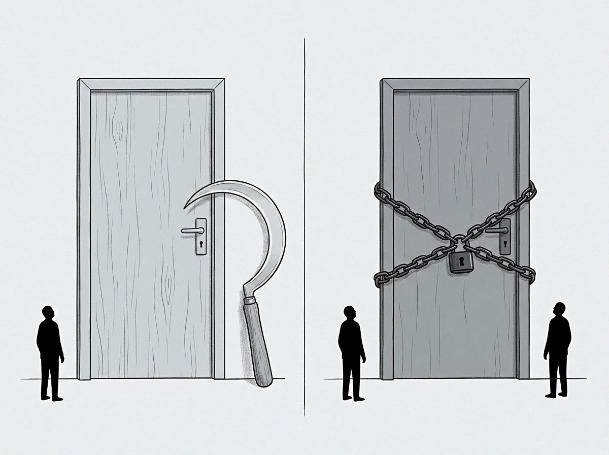
Cache
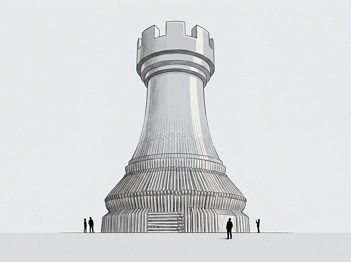
What Prevents Baseline Erosion Under Tight Windows?
The primary defense against metric decay in continuous schedules is enforcing a live computation barrier against cached tolerances. A cached answer manifests when a system substitutes an assumed distribution for empirical evaluation. Continuous deployment tools evaluating pipeline health often pull static configuration parameters—like a maximum acceptable response latency of two hundred milliseconds—and treat that ceiling as a baseline.
A ceiling is not a baseline. A ceiling marks an arbitrary boundary of gross failure, whereas a baseline defines actual empirical behavior under controlled conditions. When a service operates with a genuine baseline latency of forty milliseconds, a jump to one hundred and twenty milliseconds represents severe internal degradation.
If the pipeline relies on the cached ceiling of two hundred milliseconds, the metric registers as nominal, confusing survival below a catastrophic threshold with maintaining performance.
Preventing this erosion requires evaluating live deltas through deterministic canary execution. A fraction of incoming production traffic—or a suite of deterministic synthetic requests—passes through both the validated container and the new release candidate simultaneously. Rather than pulling a baseline from a six-month-old database record, the system computes it live on the legacy container while running the experimental candidate alongside it.
Both instances receive identical inputs under identical external conditions. Network congestion, database query locks, and client payload profiles match across both branches, leaving the computed delta purely a function of code execution variance. External environmental noise cancels out mathematically; output varies only when the software itself changes the result.
Baseline validity holds only when external environmental variance acts equally on the reference instance and the candidate instance.
Live computation requires real discipline and infrastructure overhead. Executing parallel runs doubles compute expenditure for every release test, leading budget-constrained teams to query historical telemetry databases instead. This introduces systematic sampling error: the query retrieves numbers recorded under unknown environmental variables, stripping the comparison of statistical rigor.
The shortcut appears harmless during low traffic, but breaks down completely under load spikes. When a software update releases during an unexpected traffic spike, historical metrics reflect calm conditions while the new container battles a surge. The historical telemetry cannot show whether the candidate code handles the load better or worse than the previous iteration.

Audit
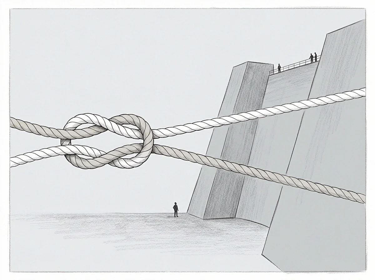
Structural Governance for Continuous Cycles
Preserving baseline telemetry across rolling release environments requires formal retrospective audits operating outside pipeline automation. Automated systems act deterministically on the rules given to them; if those rules let moving averages inform baseline values, the pipeline will automate its own progressive decline without hesitation.
An operator conducts the audit by pulling execution traces from three distinct points: the initial baseline certification run, a randomized sample from the median of the trailing quarter, and active production output. Running these three traces against an invariant benchmark test suite yields the true cardinal drift vector. If this vector exceeds acceptable tolerances, the deployment schedule freezes regardless of whether individual daily releases passed localized tests.
Engineers can debate application performance indefinitely, but measurement data settles the matter. When memory footprint per hundred requests climbs from twelve megabytes to thirty-one megabytes across forty releases, performance has degraded. High rolling frequencies disguise the trend by distributing losses across imperceptible steps; the audit surfaces this step function by collapsing intervening time.
The contract between the pipeline and the engineering organization specifies clear boundaries for baseline renewal. Recalibration occurs only when architectural changes render the previous baseline non-representative of deliberate design choices. A database engine migration is a structural change that invalidates historical query profiles; optimizing an internal JSON parser is an incremental update that must prove itself against the original baseline without moving the target.
Whether this discipline survives the operational pressure of high-frequency delivery remains an open question for engineering leadership.