
Mahalanobis Distance Modeling for Complex Multi Dimensional Production Telemetry
Mahalanobis distance detects multivariate telemetry anomalies by scaling metric deviations against empirical covariance to neutralize correlation noise.

Axis
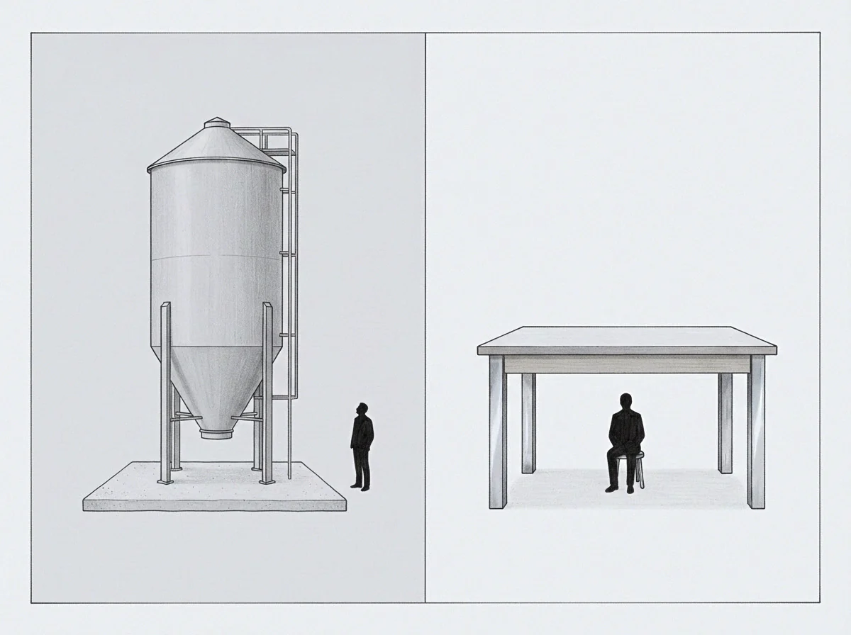
Covariance Geometry and Euclidean Blindness
Production telemetry spans dozens of co-dependent signals at any given moment. CPU utilization, memory pressure, disk write latency, request arrival rates, and database lock hold durations fluctuate together during traffic surges. Standard Euclidean distance models treat each metric as an independent, orthogonal dimension.
In that coordinate space, a joint rise in request volume and thread allocation reads as a large displacement from the origin, firing alerts even when the ratio between the two metrics matches ordinary operating equilibrium. Mahalanobis distance resolves this blindness by scaling metric offsets against the empirical covariance structure of the underlying runtime environment.
The formulation maps hyper-ellipsoids to the principal directions of system variance rather than drawing spherical distance boundaries. Euclidean distance sums unweighted squared differences across isolated signals, whereas the Mahalanobis metric projects the raw observation vector through the inverse sample covariance matrix. Each signal is normalized by historical variance, and linear dependencies between paired signals are removed.
The resulting scalar measures how many standard deviations an incoming telemetry vector falls from the multivariate center along the actual axes of observed variation.
A metric anomaly score reflects distance from the historical covariance manifold rather than absolute departure from an arbitrary scalar threshold.
The mathematical operation establishes an intrinsic coordinate system for production telemetry. Let an incoming sample vector of telemetry metrics be denoted as x, the multivariate historical mean vector as μ, and the empirical covariance matrix as Σ. The squared Mahalanobis distance D2 is computed directly:
D2(x, μ) = (x – μ)T Σ-1 (x – μ)
When two signals show strong positive correlation, an observation where one climbs while the other falls incurs a heavy penalty. That counter-directional movement cuts across the established covariance ridge, producing a high Mahalanobis distance even if both metrics remain within their individual historical min-max limits. Proportional increases along the primary axis of variance generate negligible distance shifts, suppressing false alerts during expected demand spikes.
When an identity matrix replaces the inverse covariance matrix, the expression collapses directly to standardized Euclidean distance, dropping all information about directional co-movement.
Ellipsoid

Degeneracy in High Dimensional Telemetry
Telemetry pipelines across distributed infrastructure ingest hundreds of distinct metric streams per node. As dimensionality scales, the empirical covariance matrix approaches singularity. High dimensional telemetry spaces often contain collinear metrics, such as thread pool allocations that match active request counts or mirrored block storage metrics tracking filesystem writes directly.
When two or more channels exhibit linear dependence, the determinant of the covariance matrix drops to zero, preventing direct inversion and destroying numerical stability.
Inverting an ill-conditioned covariance matrix introduces severe floating-point instability. Near-zero eigenvalues in the sample covariance matrix become massive eigenvalues in the precision matrix, turning minor high-frequency measurement noise into large artificial anomaly values. A slight sensor drift on a low-variance metric can dominate the entire distance calculation and obscure structural failures across core paths.
High dimensionality also requires substantial historical depth; estimating an unconstrained covariance matrix across p telemetry channels requires at least p(p + 1) / 2 independent parameters.
Sample covariance inversion without eigenvalue regularization guarantees numerical instability in high dimensional monitoring topologies.
The condition number of the empirical covariance matrix reflects the ratio between its maximal and minimal eigenvalues. In production systems with unpruned telemetry sets, condition numbers routinely exceed machine precision thresholds, turning routine matrix operations into persistent sources of false alerts.

Wall

Theoretical Thresholds Against Empirical Drift
Assuming multivariate normality in the underlying telemetry distribution, squared Mahalanobis distance follows a Chi-squared distribution with degrees of freedom equal to the count of modeled metric dimensions. Under this baseline, statistical anomaly thresholds are set by evaluating the cumulative distribution function at a target significance level, such as selecting a ninety-nine percent critical value to isolate outliers. Real infrastructure metrics diverge from this assumption, showing heavy tails, multimodal states, and asymmetric bursts during autoscaling events.
| Evaluation Vector | Euclidean Distance Baseline | Mahalanobis Production Model | Shrinkage Regularized Model |
|---|---|---|---|
| Signal Correlation Sensitivity | Zero correlation tracking across dimensions | Full linear covariance alignment | Full covariance with bounded noise amplification |
| Alert Resilience to Load Surges | Low resilience with frequent false positives | High resilience along correlated axes | High resilience with minimal boundary drift |
| Dimensional Scalability Limit | Arbitrarily high without matrix inversion | Constrained by matrix singularity threshold | Extended to high dimensional spaces via shrinkage |
| Computational Complexity per Point | Linear time O(p) across channels | Quadratic time O(p^2) with precomputed inverse | Quadratic time O(p^2) with stable online updates |
The boundary between normal variance and active degradation moves throughout diurnal traffic cycles. Applying a static Chi-squared cutoff to non-Gaussian telemetry produces systematic blind spots during low-load intervals and alert storms during sudden traffic shifts. Tuning the detection threshold requires bounding empirical tail behavior directly rather than relying on theoretical Chi-squared quantiles.
- Covariance Matrix Regularization bounds the minimal eigenvalue of the dispersion matrix, preventing inverted noise artifacts from corrupting distance scores in high dimensions.
- Sliding Window Estimation discards stale operational baselines, tracking structural changes across software release boundaries.
- Dimensionality Compression projects correlated metric clusters onto lower dimensional orthogonal manifolds prior to distance calculation, eliminating exact linear dependencies.
- Empirical Quantile Calibration replaces rigid Chi-squared distribution assumptions with non-parametric percentiles derived from verified operational baselines.
A detection model calibrated on high-load diurnal patterns treats low-load anomalies with reduced sensitivity, allowing memory leaks during off-peak windows to progress unchecked.

Shrinkage
Conditioning Matrices for Continuous Streaming
Maintaining numerical stability across live metric streams requires continuous conditioning. Ledoit-Wolf shrinkage stabilizes the empirical sample covariance matrix by pulling it toward a well-conditioned target, such as a diagonal matrix with equal variance across all axes. The shrinkage estimator calculates an optimal interpolation weight that balances sample variance against structural bias, keeping the matrix positive definite and invertible across operating shifts.
Streaming architectures avoid recalculating full matrix inverses on every metric tick by applying the Woodbury matrix identity or rank-one Cholesky factor updates. As new telemetry arrives, historical mean and covariance matrices update through an exponential decay factor, letting the baseline track architectural drift without full inversions. The inverse covariance matrix updates in quadratic time, supporting low-latency evaluation on high-frequency streaming infrastructure.
Online Cholesky factor updates allow real-time Mahalanobis scoring without repeated cubic-time matrix inversions on ingestion paths.
Consider a pipeline tracking four core infrastructure metrics across a distributed storage cluster: disk input-output operations per second, memory allocation delta, read queue length, and write serialization delay. Under an unregularized empirical covariance model, temporary lock contention causes write latency to spike while disk operations drop to zero, pushing the sample covariance matrix close to singularity. Applying a regularized shrinkage estimator keeps the precision matrix eigenvalues bounded, allowing the distance metric to isolate the counter-correlated lock contention event without numerical overflow.

Is Linear Covariance Sufficient for Non-Linear Production States?
Microservice architectures undergo nonlinear state transitions that exceed the capacity of a single global covariance matrix. A service moving from thread-based execution to an asynchronous event loop shifts its operational manifold, altering the linear correlations present in earlier deployment cycles. Under architectural shifts of this scale, calculating distance against a static covariance center introduces steady model error.
Engineering teams handle this drift by maintaining localized covariance clusters or applying streaming kernel approximations when operating states move away from unimodal geometry.
Relying on a single global covariance matrix across distinct operational modes guarantees elevated false negative rates during unrepresented system states.
Seat

Operational Deployment in High-Throughput Pipelines
Deploying Mahalanobis distance scoring in real-time alerting systems requires separating baseline generation from evaluation. The baseline worker processes historical metric archives asynchronously, generating regularized precision matrices and empirical distance thresholds across rolling time windows. The ingestion worker receives live telemetry vectors, normalizes them against the active baseline mean, and runs the vector-matrix-vector multiplication in memory via optimized BLAS routines.
This separation isolates the evaluation pipeline from processing bottlenecks. A single telemetry node emitting hundreds of metrics per second evaluates its distance in microseconds, passing a scalar health indicator to alerting engines. Downstream consumers treat the result as a unified multivariate anomaly indicator, initiating diagnostics only when an observation vector exits the empirical threshold envelope.
When an anomaly surfaces, decomposing the Mahalanobis distance vector isolates the specific metric pairs contributing most of the variance, identifying the exact correlation breakdown.
The operational cost of maintaining multi-dimensional telemetry models centers on the continuous calibration of baseline windows against infrastructure evolution.