
Reconstructing Latent Dimensional Collapse When Operational Telemetry Fails To Track Phase Transition Boundaries
Latent dimensional collapse occurs when state space variables align into reduced manifolds prior to phase transition while scalar telemetry reports static averages.

Floor
An operator can watch a dashboard where every primary operational scalar sits comfortably within baseline limits, even as the system’s underlying state distribution narrows into a restricted subspace. Conventional telemetry monitors performance indicators in isolation through univariate variance, average throughput, and local latency caps. These direct readouts gauge surface volume without evaluating cross-variable correlation.
Dynamics near a phase transition boundary show distinct shifts in variance structure while aggregate averages stay flat. Operating capacity looks steady until the multi-variable equilibrium breaks.

Scalar Telemetry Masking Dimensional Compression
Monitoring architectures built on isolated sensor boundaries assume orthogonal state variables. Production infrastructure, however, develops dense coupling across layers, linking memory allocation, queue depth, disk operations, and network saturation. As external load climbs or internal contention spreads, system flexibility narrows because variable dependencies begin to align.
The overall state space contracts into a smaller volume. Individual gauges show nominal health while latent flexibility drains away.
System capacity degrades silently when scalar metrics isolate individual dimensions from multi-variable alignment.
High-dimensional infrastructure relies on structural dispersion for stability. So long as operational degrees of freedom stay independent, localized shocks bleed off along redundant execution paths. Sustained environmental load eventually forces separate variables into lockstep, triggering latent dimensional collapse ahead of any physical breakdown.
Telemetry channels post a zero anomaly score because statistical thresholds evaluate single metrics rather than mutual information. The lower boundary of system variance simply caves in.
Overlooking multi-variable variance decay leaves teams unprepared for sudden phase shifts. Workload volume continues to scale based on aggregate health metrics, but downstream services lose structural buffers well before scalar thresholds trip an alert. The eventual disruption hits without preliminary univariate warning.
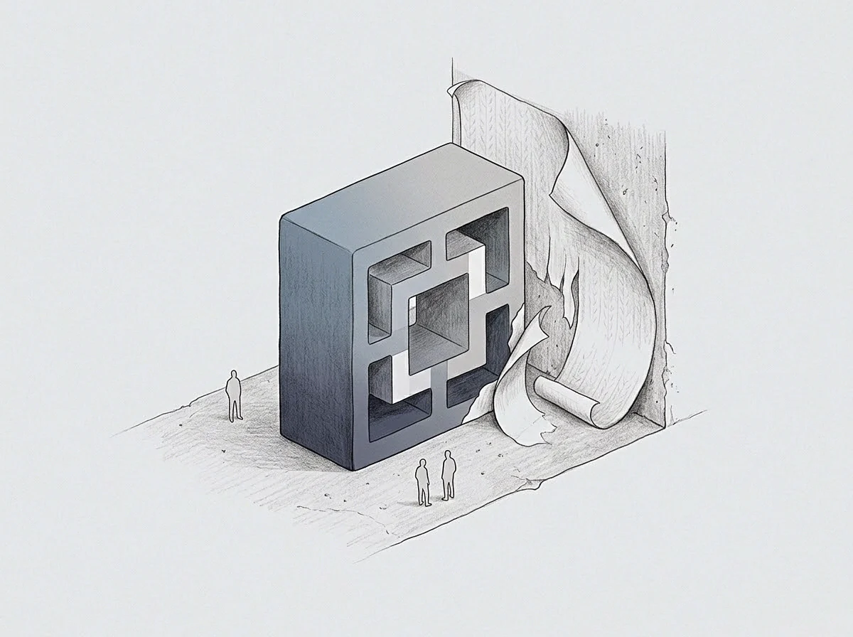
Decay
Spectral density shifts across state vectors point to structural decay long before a failure takes place. When an operating environment drifts toward a bifurcation point, the time required to recover from minor operational shocks lengthens. This behavior, known as critical slowing down, shows up as higher autocorrelation between successive collection intervals.
Standard telemetry aggregation flattens these micro-fluctuations, mistaking systemic sluggishness for steady execution.
How Do Unmonitored Cross Covariances Force Critical Slowing Down?
Subtle inter-variable alignment accelerates structural degradation while baseline scalar dashboards stay green. Calculating a complete covariance matrix across hundreds of runtime metrics requires computational overhead that real-time collection pipelines often avoid. Routine sampling drops high-frequency phase detail to save ingestion bandwidth, discarding the dynamic signature of an impending collapse.
Four primary structural changes characterize latent variance erosion across unmonitored system dimensions:
- Covariance Inflation occurs when previously uncorrelated state variables begin moving in tight synchronization during routine load distribution variations.
- Autocorrelation Persistence extends the temporal recovery baseline, causing system noise to linger across successive telemetry polling cycles.
- Variance Asymmetry skewness shifts state distribution density toward physical operating limits without shifting the calculated median value.
- Spectral Concentration concentrates structural energy into a single dominant principal component as residual degrees of freedom collapse.
State variance condenses under ongoing operational strain. Calculating effective degrees of freedom shows how many independent avenues remain to absorb unexpected friction. When a system operates with reduced variance modes, it loses the internal padding needed to handle routine transient spikes.
Persistent cross-variable correlation reveals structural decay long before scalar thresholds cross operational limits.
Architectures under continuous load tend to follow paths toward state compression. Systems optimized purely for steady-state throughput drift into tightly coupled trajectories. Pushing for maximum efficiency flattens dimensional range, exchanging structural resilience for immediate output.

Manifold
Pinpointing hidden dimensional loss requires charting the low-dimensional manifold where state vectors congregate. When high-dimensional space collapses, operational trajectories slide toward a narrow hypersurface set by systemic limits. Reconstructing this geometry after an incident means analyzing residual variations and off-diagonal covariance terms.
Because standard telemetry drops off-diagonal data, engineers must rebuild these structures from asynchronous transaction logs.
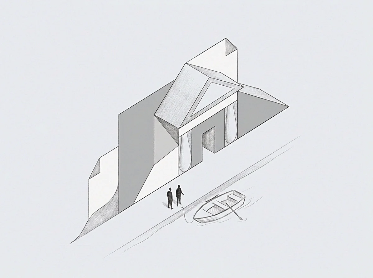
Eigenvalue Collapse Along Primary State Vectors
Spectral decomposition of historical telemetry records exposes the drop in operational degrees of freedom. In principal component analyses run across sliding time windows, the eigenvalue spectrum reveals energy gathering rapidly in the leading components. The remaining eigenvalues shrink toward zero, indicating that system variance has aligned along a single constrained vector.
This spectral narrowing marks the true boundary of early phase transitions.
Maintaining visibility into stability depends on sustained computation across state spaces. Monitoring infrastructure struggles when structural analysis requires intensive matrix calculations rather than basic time-series lookups. Reading scalar values takes minimal compute, whereas rebuilding state manifolds in real time demands continuous numerical processing at scale.
Telemetry Versus Spectral Reconstruction Matrix
The difference between standard operational telemetry and spectral reconstruction methods determines whether an engineering team detects latent boundary transitions or suffers unannounced service disruption.
| Evaluation Dimension | Standard Operational Telemetry | Spectral Manifold Reconstruction |
|---|---|---|
| Measurement Focus | Univariate scalar magnitudes and thresholds | Multivariate state covariance structures |
| Sampling Strategy | Periodic static polling intervals | Continuous trajectory snapshot streaming |
| Early Warning Window | Zero lead time prior to boundary breach | Significant lead time during variance decay |
| Compute Overhead | O(N) linear scalar evaluation cost | O(N squared) matrix covariance processing |
| Sensitivity Range | Detects explicit threshold violations | Detects subtle dimensional compression |
A typical production incident illustrates the hidden mechanics of manifold collapse. Take a microservices cluster handling transaction volume across thirty decoupled node instances. Assume database connection pools, queue depths, and memory usage are recorded every ten seconds.
Over a six-hour operational shift, scalar CPU usage remains stable at sixty-five percent, while network saturation sits at forty percent. Under standard telemetry rules, no alert fires.
Deeper analysis shows a different reality. The correlation between database connection latencies and garbage-collection cycles climbs from a baseline of zero point twelve to zero point eighty-seven. The available state space collapses from thirty independent operational variables into two coupled operational vectors.
When a brief five percent load spike hits the system, the lack of orthogonal buffer pathways causes an immediate cascade of connection timeouts across all nodes simultaneously. Telemetry failed because sensors evaluated isolated scalar values rather than the geometry of the manifold.
An operational system running with reduced spectral dimensions converts minor transient noise into full failure cascades.
Uptime agreements focus on performance caps rather than variance boundaries. Standard operating contracts track availability percentages while overlooking markers of structural resilience. Safety erodes quietly whenever service metrics meet contractual targets while internal variance collapses.

Proxy
When primary metrics fail to capture internal state shifts, analysis depends on shadow telemetry drawn from secondary signals. High-frequency noise, inter-arrival time distributions, and residual compute variances serve as structural proxies. These secondary indicators reflect the friction generated as state vectors push against unmapped stability boundaries.

Deriving Shadow Metrics From Higher Order Residuals
Isolating proxy measurements requires separating structural indicators from background system noise. Standard data pipelines smooth out high-frequency fluctuations using moving averages. Reconstruction workflows invert that approach, treating residual variations as primary diagnostics.
The amplitude of residual noise grows predictably as the environment nears a phase threshold.
Reconstructing structural collapse from secondary proxy signals follows an explicit sequential path:
- Isolate high-frequency residual noise by subtracting smoothed trendlines from raw operational streams.
- Compute sliding window variances across residual series to measure localized signal variance expansion.
- Extract higher-order statistical moments including skewness and kurtosis from residual distributions.
- Construct surrogate cross-correlation matrices across proxy metric streams to monitor signal alignment.
- Calculate the effective topological dimension of the reconstructed state space to verify manifold shrinkage.
Secondary proxy metrics show the true cost of operating near stability limits. Stripping out operational headroom creates severe structural brittleness that cancels out immediate efficiency gains. Ingestion pipelines bypass high-frequency calculations to keep transport costs low, introducing hidden systemic risk in the process.
Reconstructing system trajectories from residual noise exposes structural stability limits that scalar gauges hide.
Downstream service response times often appear normal until complete failure occurs, and standard SLA metrics give no early warning before an interruption. Service level agreements evaluate output delivery rather than internal structural health.

Remnant
Post-incident analysis relies on examining the trajectory remnant preserved in historical event logs after a phase transition. During a sudden state shift, primary monitoring tools frequently drop frames or truncate disk writes. Reconstructing the failure path requires assembling asynchronous traces, kernel audit records, and hardware interrupt logs.
These low-level artifacts preserve the final direction of the state vector.

Mapping Trajectory Memory Across Boundary Passages
System state retains residual physical orientation through rapid phase changes. Non-volatile cache entries, socket buffer queues, and unwritten log buffers hold the geometric orientation of state vectors at the moment of breakdown. Evaluating these remnants allows engineers to reconstruct the exact shape and angle of the critical manifold.
State transitions leave clear directional markers in execution remnants. By calculating the trajectory of maximum velocity through state space during failure, analysis isolates the coupling mechanism that caused the shift. This mapping converts an operational failure into actionable boundary coordinates.
A single operational question remains open following post-collapse reconstruction. What minimal subset of continuous cross-covariance computations must be embedded directly into hardware telemetry pipelines to guarantee real-time detection of dimensional collapse before boundary passage occurs?