
Standardizing Multi Axis Vector Trajectories Through Statistical Score Normalization
Statistical score normalization transforms disparate metric axes into an isotropic vector space, eliminating scalar variance dominance to track true multi-axis operational trajectories.

Scale
An operational dashboard tracking performance frequently displays distinct metrics side by side without mathematical reconciliation. A quarterly budget variance measured in hundreds of thousands of dollars sits adjacent to a single-digit software defect rate or an ordinal customer sentiment score. When an operator attempts to combine these parameters into a unified trajectory vector, the mathematical magnitude of the financial figure swallows the movement of the smaller metrics.
The geometric consequence of unadjusted multi-axis measurement is immediate. In an N-dimensional operational space where each axis represents a separate performance variable, distance calculations rely on the Euclidean norm. If one axis possesses a variance several orders of magnitude wider than its neighboring axes, any calculated trajectory vector simply mirrors the fluctuations of that dominant axis.
Directional shifts along narrower axes become invisible, regardless of their operational urgency.
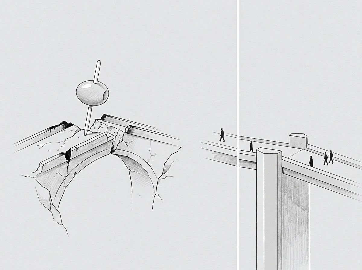
Anisotropic Distortion Across Unmatched Metric Axes
Anisotropy in metric spaces occurs when physical or numerical distances carry unequal weight depending on the directional axis measured. An operational trajectory moving through raw score space undergoes continuous severe distortion, where scalar volume overrides directional movement.
Consider an engineering organization tracking three concurrent metrics: monthly server deployment velocity, software defect resolution time, and developer retention rate. Server deployment counts range from forty to two hundred units per month. Defect resolution averages three to six days.
Retention rate moves within a narrow band between zero point eight five and zero point nine eight. Unnormalized vector aggregations treat a change of fifty deployment units as fifty times more significant than a full point zero five drop in retention. The system routes around the subtle erosion of retention because the deployment metric exerts total geometric dominance over the trajectory calculation.
A multi-axis trajectory retains true directional slope only when each constituent axis operates within an identical variance boundary.
Standardizing trajectory vectors requires forcing every measured axis into a common dimensionless scale. Without statistical score normalization, multi-axis tracking acts as a single-variable display disguised as a multi-dimensional control signal.

Mathematical Principles of Multi Dimensional Trajectory Projection
Statistical score normalization translates raw metric inputs into standardized representations, typically centered at zero with a unit standard deviation. The standard normal transformation subtracts the sample mean of an axis from each raw observation and divides the result by the sample standard deviation. This operation maps disparate operational scales onto a unified isotropic coordinate system where a one-unit displacement along any axis reflects an identical statistical departure from expected baseline performance.
When an operator maps normalized score vectors across successive time steps, the resulting trajectory accurately reflects multi-axis momentum. The path length in normalized vector space measures genuine organizational movement rather than scalar volume. Failing to apply statistical standardization to multi-axis trajectory vectors leads directly to misallocated operational effort, as resource allocation engines dynamically optimize for scalar volatility while structural decay on narrow axes proceeds undetected.

Window
Calculating statistical score normalization demands choosing an explicit lookback period for computing the sample mean and standard deviation. The baseline interval defines the memory of the analytical engine. Choosing a static twelve-month baseline establishes an anchored reference frame, whereas a rolling thirty-day lookback frame adapts dynamically to recent operational conditions.
A static baseline loses descriptive accuracy as operational baselines shift over time.
The trade-off between static and dynamic normalization frames governs system responsiveness. A static baseline highlights long-term organizational drift relative to a fixed historical benchmark. It struggles, however, when operational paradigms shift permanently, causing normalized scores to sit continuously at structural extremes.
A rolling dynamic baseline adapts to operational shifts, but risks normalizing chronic underperformance by continuously integrating deteriorated metrics into the baseline average.

Rolling Statistical Normalization and Temporal Baseline Hysteresis
The chosen observation window establishes the calculated trajectory slope.
When an analytical system utilizes a rolling window to normalize multi-axis vectors, baseline hysteresis introduces subtle feedback loops. Hysteresis occurs when the current standardized value of a metric depends strongly on the temporal path taken to reach it. A sudden spike in operational costs temporarily inflates the rolling standard deviation denominator for subsequent periods.
As a result, subsequent cost fluctuations appear artificially dampened in the standardized trajectory, masking continued structural instability.
Extending the baseline frame beyond three operational cycles suppresses genuine trajectory shifts under historical statistical inertia.
Managing dynamic statistical frames requires explicit operational choices regarding lookback length and weighting decay functions. Exponentially weighted moving averages grant greater influence to recent operational states, allowing the standardized trajectory to reflect real-time directional shifts while retaining statistical stability against transient noise.
The failure modes associated with temporal normalization windows fall into three primary categories:
- Baseline Saturation occurs when recent high-variance spikes suppress subtle systemic motion across secondary axes by artificially inflating the rolling standard deviation denominator.
- Lagged Vector Orientation happens after swift operational corrections because historical statistical scores linger in the lookback frame, pulling the current direction toward past states.
- Variance Compression limits the visibility of intentional strategic turns by expanding the variance denominator during volatile operational phases, flattening the apparent magnitude of intentional moves.

State Transitions in Shifting Variance Envelopes
Operational environments transition through distinct variance regimes. A period of steady-state execution exhibits narrow standard deviations across most operational metrics, followed by high-volatility phases during platform migrations or structural restructurings. Normalizing vector trajectories across a regime change breaks simple linear assumptions.
If an organization enters a high-volatility regime while retaining a narrow baseline standard deviation from a previous steady-state phase, normalized scores explode in magnitude. Trajectory vectors hit extreme coordinates, triggering false alarm thresholds across automated control loops. Stating the temporal window length alongside the specific variance bounds within contract agreements prevents misinterpretation of standard score trajectory spikes during planned regime transitions.

Clock
Temporal alignment presents a major obstacle when standardizing multi-axis trajectories. Metrics within an operational ecosystem refresh at distinct frequencies. Financial ledger entries update monthly, customer churn data aggregates weekly, API latency figures generate every millisecond, and employee sentiment scores publish quarterly.
Fixed chronological intervals measure elapsed time rather than operational progression.
Constructing a synchronized multi-axis trajectory vector requires imposing a unified cadence across asynchronous metric streams. Interpolating slow metrics between update cycles risks introducing phantom trajectories that do not correspond to real operational events. Conversely, downsampling high-frequency data to match slow cadence metrics discards valuable high-frequency vector momentum information.

Temporal Cadence and Velocity Vector Alignment
Asynchronous logging intervals conceal underlying vector drift across operational domains.
Aligning asynchronous metric axes demands treating trajectory tracking as an event-driven system rather than a time-driven clock. Instead of sampling metrics at fixed calendar hours, system states trigger vector evaluations upon reaching specific state transitions or transactional volumes. Event-based sampling ensures that trajectory calculations capture real operational work rather than temporal passage.
- Sample every operational vector at uniform state updates rather than fixed temporal ticks.
- Calculate local variance across a bounded sequence of active state changes.
- Re-project the trajectory vector against the updated standard deviation matrix.

When does vector trajectory scaling collapse?
Scaling collapses when temporal sampling intervals diverge past the operational decay rate of the metric being tracked. If a metric undergoes complete internal variance turnover within twenty-four hours, sampling it on a weekly cadence renders statistical normalization meaningless. The calculated mean and standard deviation no longer represent the active state envelope, causing the standardized score to reflect historical artifact rather than current trajectory.
Sampling multi-axis vectors at event transitions rather than temporal ticks isolates true mechanical momentum from passive duration.
Maintaining trajectory validity requires matching the normalization sampling rate strictly to the shortest structural coherence window among all constituent metrics. A trajectory remains robust only so long as the temporal gap between metric samples stays shorter than the time required for underlying operational conditions to reset completely.

Matrix
Selecting an appropriate mathematical transformation determines how effectively score normalization preserves genuine trajectory signals while suppressing non-systemic anomalies. Standard score z-scoring, robust percentile scaling, and Mahalanobis distance vector transformations handle extreme values and cross-axis correlations differently.
The transformation matrix provides the coordinate system for comparing disparate metrics.
Z-score normalization relies on Gaussian assumptions, utilizing the parametric mean and standard deviation. When operational metrics exhibit heavy-tailed distributions or extreme outliers, z-score transformations compress typical operational variance into narrow bands, while outliers dominate the normalized axis. Robust scaling replaces the mean with the median and the standard deviation with the interquartile range, insulating the multi-axis trajectory from single-event distortions.
Unadjusted variance across metric distributions conceals underlying rate-of-change momentum.

Comparative Evaluation of Trajectory Normalization Methods
Evaluating normalization methods requires examining their sensitivity to extreme values, computational overhead, and capacity to handle cross-axis variance correlations. The comparison below outlines structural characteristics across the three primary vector standardization techniques.
| Normalization Method | Mathematical Formulation | Sensitivity to Extreme Outliers | Computational Complexity | Primary Operational Use Case |
|---|---|---|---|---|
| Z-Score Standardization | Subtraction of parametric mean divided by sample standard deviation | High: outlier values expand denominator and pull the mean | Low: basic linear arithmetic across scalar dimensions | Symmetric Gaussian metric distributions with stable baseline bounds |
| Robust Percentile Scaling | Subtraction of median divided by Interquartile Range | Low: extreme values leave median and interquartile range intact | Moderate: requires sorting operations to calculate percentiles | Heavy-tailed operational distributions with frequent transient spikes |
| Mahalanobis Vector Scaling | Square root of covariance-weighted Euclidean distance vector product | Moderate: sensitive to covariance matrix instability | High: matrix inversion and covariance calculations required | Correlated multi-axis metric spaces with interdependent cross-variance |
| Source: Desk reference on trajectory standardization and multi-axis score normalization mechanics. | ||||
Mahalanobis distance normalization extends standardization by incorporating the covariance matrix between operational axes. Standard z-score and robust percentile scaling treat each metric axis as independent, assuming orthogonal dimensions. Operational metrics, however, rarely operate in isolation.
Cash burn rate and engineering headcount growth frequently exhibit strong positive covariance.
An unadjusted variance denominator converts temporary operational spikes into permanent spatial trajectory distortions.
Ignoring cross-axis covariance leads to double-counting shared variance along correlated dimensions. The Mahalanobis transformation decorrelates the metric axes while normalizing variance, projecting the trajectory into a true orthogonal vector space. This operation reveals the underlying directional trajectory free from redundant multi-metric signals.
An unadjusted dashboard suggests that two parallel metrics rising simultaneously prove double the strategic momentum, whereas covariance normalization demonstrates that only a single operational force is active.

Drift
Statistical score normalization operates on the foundational assumption that operational metrics move within bounded, statistically discoverable distributions. Regime shifts violate this assumption. A regime shift occurs when an organization fundamentally changes its operational model, rendering historical statistical parameters irrelevant.
Isolated anomalies skew historical mean calculations across the evaluation window.
When a software enterprise transitions from self-hosted software sales to a recurring cloud service model, metrics such as cash collection velocity, customer support volume, and infrastructure provisioning cost undergo permanent structural step-functions. Continuing to normalize new operational vectors against pre-transition means and standard deviations produces perpetual extreme z-scores. The standardized trajectory hits the structural limit of the earlier statistical model.

Non Gaussian Regime Shifts and the Model Boundary
Statistical normalization breaks down when operations shift outside assumed Gaussian distributions.
This limit marks the boundary of statistical score normalization. When an operational metric distribution enters non-Gaussian regimes characterized by power-law dynamics, standard score normalization fails entirely. In a power-law environment, sample variance does not converge to a stable population variance as sample size increases.
Calculating a standard deviation denominator becomes mathematically unstable, causing normalized trajectory vectors to wander randomly based on sample size choices.
Unadjusted statistical divergence compounds across successive projection steps.
Recognizing the model boundary requires continuous testing for distribution normality and stationarity. When variance tests signal power-law behavior or non-stationarity across key operational axes, standard score standardization must be paused. The engine shifts to non-parametric percentile mapping or ordinal ranking mechanisms to prevent false trajectory vectors from misguiding executive decision loops.

Latent Vector Mirroring Above the Standardized Baseline
A system continuously routing around a specific operational domain leaves a distinct signature within normalized vector space. The unaddressed operational area acts as a coordinate marker. If an organization systematically avoids addressing technical debt or renegotiating legacy customer contracts, those neglected dimensions sit at persistent negative standardized score positions while active dimensions absorb operational energy.
Mirroring the negative trajectory vector above the baseline reveals the latent capacity of the system. The unspent volume sitting behind the avoided operational axis carries a magnitude equal and opposite to the historical avoidance vector. Standardizing multi-axis vectors isolates these structural asymmetries, stripping away scalar noise to highlight precisely where unprocessed operational friction accumulates behind organizational constraints.
When an operational team identifies an axis holding a persistent negative normalized score while neighboring axes operate at elevated positive levels, the slope indicates a structural bottleneck rather than an execution failure. The team resets the baseline window to the precise timestamp of the last operational shift, recalibrates the covariance matrix across active axes, and tracks the trajectory vector as it crosses the zero-score baseline into positive territory.