
Calculating Thermal Hysteresis Variance Vectors Between Cached Engineering Models and Post-Close Operational Load
Calculates deviation between static thermal models and operational plant cooling lag by mapping empirical temperature paths against invariant reference projections.
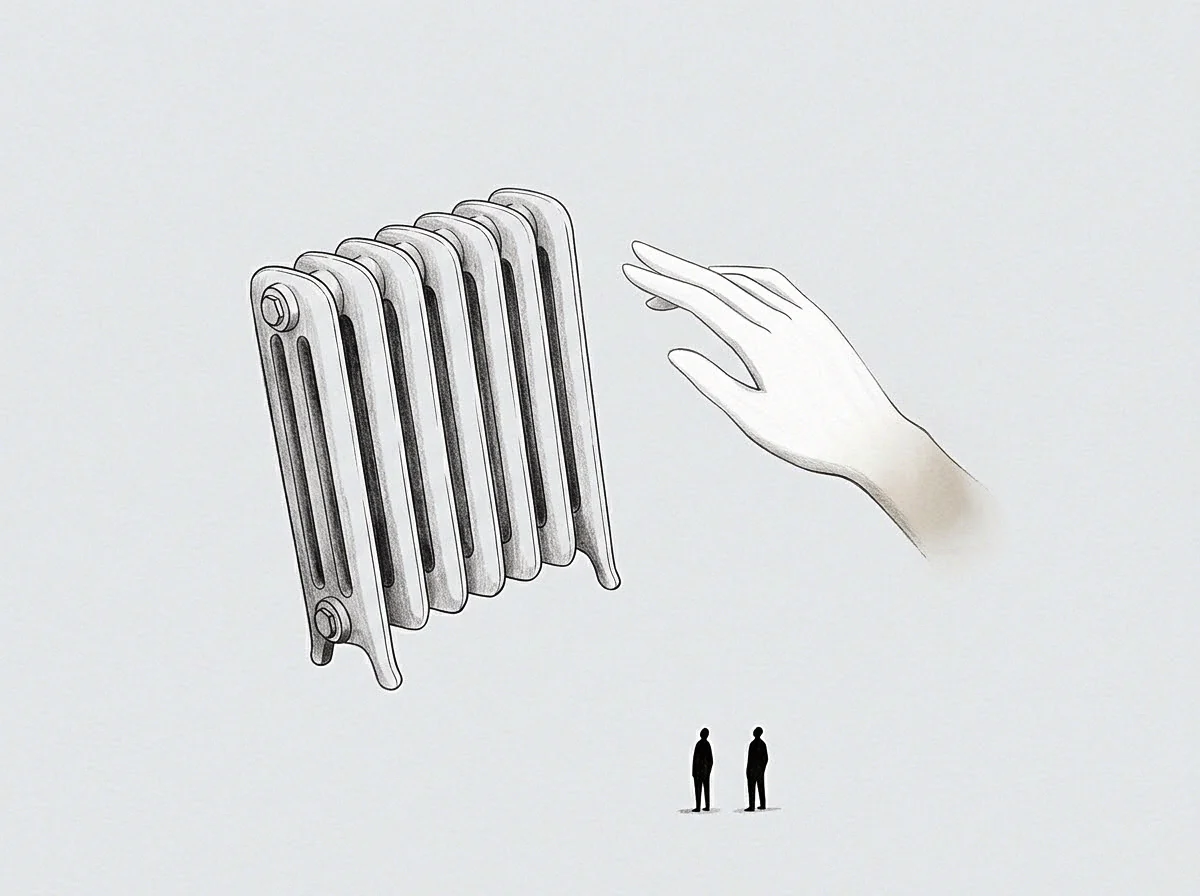
Furnace
An asset acquisition closes on paper, yet the physical machinery often runs colder than the investment prospectus modeled. Engineering spreadsheets project steady dissipation rates, drawing clean thermodynamic curves where heat loss maps linearly against output. On the factory floor, cooling cycles stretch across irregular operational hours, retaining internal energy and shifting structural clearances long before a maintenance crew logs the deviation.
This divergence between static projections and dynamic plant performance marks the thermal hysteresis variance. Thermal hysteresis describes the lag between heat intake and subsequent mechanical relaxation, where material history dictates subsequent operational states. While simulations cached during pre-acquisition scrutiny assume steady equilibrium, daily production operates dynamically: spikes inject heat, brief shutdowns pull the baseline down unevenly, and the variance vector between modeled and observed thermal behavior widens with every shift cycle.
A thermal hysteresis variance vector records the path dependence of energy dissipation across variable manufacturing cadences.
Plant teams inherit both the model and the machinery. Treating cached engineering assumptions as absolute baselines introduces operational vulnerability across the facility. Where the spreadsheet assumes thermal recovery follows a reversible path, the physical assembly, worn by cumulative cyclic strain, dissipates heat along an asymmetric loop.
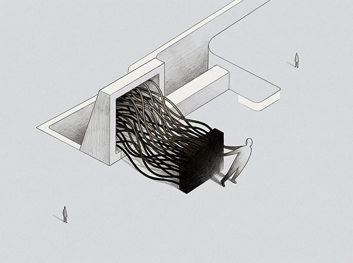
Predictive Baselines and Physical Disparity
Engineering files stored in project data rooms regularly rely on lumped capacitance assumptions. These documents model high-output compressors, extrusion cylinders, and chemical vessels as uniform physical blocks that warm and cool across balanced curves. In practice, assemblies consist of joined alloys, composite insulation, mechanical seals, and dynamic fluids, all retaining heat along separate internal boundaries.
Forty-eight hours post-close, an operator reviewing temperature readouts finds ninety degrees Celsius at the exhaust housing while internal flange zones remain elevated at one hundred and forty degrees. The engineering model logged total thermal dissipation within four hours of idle time, yet the physical plant requires fourteen hours to shed its thermal load down to ambient equilibrium. Restarting production during this unaccounted window forces materials into structural stress regimes that the spreadsheet treated as impossible.
When engineering projections omit material thermal memory, operational scheduling forces machinery into premature loading cycles.
Path
Calculating the hysteresis variance vector requires mapping two separate paths across thermal state space. The first path traces the cached engineering projection; the second tracks empirical plant performance over continuous operational windows. Calculating the vector extracts the direction and magnitude of deviation between these trajectories at discrete points in time.
Mathematical representations of this variance evaluate the area contained within the real hysteretic loop against the flat response line predicted by historical engineering models. While the cached model serves as an invariant reference, physical operations expose the assembly to variable cycling, moisture contamination, fouling layers, and dynamic throughput.
Decomposing the Hysteresis Variance Equation
The calculated variance vector separates into two distinct scalar quantities: path directionality and relaxation delay. Let the predicted thermal trajectory be mapped as a function of operational load over time, and let live instrumentation record empirical wall temperatures across matching load intervals. The difference between these states forms the instantaneous error signal.
Continuous thermal cycling changes the geometry of the hysteresis loop itself. Under light duty cycles, internal thermal gradients remain shallow. Heavy operational demands generate steep internal thermal differentials, altering the structural resistance of components and widening the variance vector.
The variance vector expands when mechanical assemblies absorb rapid thermal charges without completing relaxation baselines.
The following sequence traces the mathematical formulation used to calculate the hysteresis variance vector from raw field telemetry:
- Baseline normalization establishes the ambient plant baseline temperature and operational setpoints recorded inside inherited engineering documentation across sixty continuous operating cycles.
- Transient tracking logs real-time thermocouple data across key structural points during rapid post-close throughput spikes and unexpected emergency shutdowns.
- Phase alignment pairs predicted thermal saturation timestamps with physical peak temperature readouts to quantify operational time lag.
- Vector extraction calculates the directional divergence between modeled and empirical heat dissipation paths across discrete load increments.
Calculations that omit directional path history misclassify chronic mechanical resistance as simple measurement noise.
Seam
Material joints, bearing housings, and structural welds bear the primary burden of thermal lag. In composite assemblies, differing expansion coefficients turn thermal hysteresis into an active mechanical risk. Joined dissimilar materials retain energy at divergent rates, twisting internal interfaces while surface sensors display normal thermal conditions.
This imbalance concentrates along the mechanical seams of major equipment. In a turbine where a cast iron housing bolts to a forged alloy steel rotor shaft, the cast iron sheds heat quickly through its porous walls. The alloy shaft retains thermal energy along its core, cooling slowly over extended rest periods.
Inherited engineering files declared the entire turbine unit fully stabilized within six hours of shutdown.
Restarting operational drive motors at hour seven binds the assembly. The internal shaft remains thermally expanded, while the outer casing has contracted to cold baseline dimensions. The resulting mechanical interference destroys internal bearings, strips copper seals, and stalls high-voltage drives.
Maintenance teams often attribute the failure to inadequate lubrication, overlooking the thermal lag that warped internal clearances.

Comparative Dynamics Across Plant Architectures
Operating environments produce distinct hysteresis signatures depending on cooling media, mechanical containment, and daily cadence. Cached spreadsheets standardize these interactions, smoothing over critical mechanical distinctions.
| Assembly Type | Cached Model Dissipation Curve | Empirical Operational Dissipation Curve | Dominant Variance Vector Driver |
|---|---|---|---|
| High-Pressure Extrusion Barrels | Symmetric logarithmic decay over 180 minutes | Asymmetric stepped retention over 520 minutes | Polyester degradation and barrel wall insulation coking |
| Continuous Chemical Digestors | Linear thermal loss tied strictly to ambient delta | Non-linear hysteresis driven by interior vessel scale | Mineral scaling acting as an unplanned thermal capacitor |
| Rotary Turbine Compressors | Uniform radial dissipation across rotor and casing | Differential core retention with casing shrinkage | Mismatched thermal expansion coefficients in alloy pairs |
| Heavy-Duty Gear Reduction Units | Immediate heat release upon oil pump recirculation | Extended thermal trapping inside gear teeth cores | Viscosity thinning and boundary-layer thermal boundary drag |
Ignoring interface dynamics along mechanical seams leads to bearing failure within the initial operational quarter.
Scale
Thermal hysteresis compounds across an industrial facility. A single unmonitored compressor running an extended cooling curve disrupts downstream condensers, alters cooling water balance, and increases overall utility expenditures. Scale turns local thermal variance vectors into facility-wide operational drag.
A plant acquisition involves financial projections predicated on nameplate efficiency, which derives from the cached engineering model. When real equipment requires forty percent more idle time to reach thermal equilibrium between batches, production velocity drops. Operators face an operational trade-off: allow the required thermal relaxation window and miss output targets, or force the restart and damage plant assets.
Consider a chemical processing facility operating six batch reactors. The investment model assumed sixteen batches per week per reactor, totaling ninety-six weekly runs. That cadence assumed reactors reach ambient conditions within ninety minutes of cleaning flushes.
Real plant telemetry reveals an internal vessel wall temperature that hovers thirty-five degrees above model parameters for three full hours.
Would Operational Cadence Survive True Thermal Measurement?
The plant cannot achieve ninety-six runs without scorching raw ingredients against hot reactor walls. The operator slows production to seventy-two runs per week to preserve batch purity, dropping output twenty-five percent below the acquisition model. Reviewing monthly performance, asset owners attribute the variance to execution failure, unaware that physical heat transfer constraints preclude the modeled schedule.
Field teams routinely attempt to mitigate thermal lag by forcing cooling cycles. Spraying cold process water onto hot structural surfaces induces thermal shock. Cold air blasts cause outer metal skins to contract while interior cores remain expanded.
The resulting micro-fractures compromise equipment pressure boundaries long before routine ultrasonic testing detects the fault.
These structural strains generate unbudgeted depreciation costs that never appeared in pre-acquisition models.

Drift
Over months of operational ownership, the hysteresis variance vector drifts continuously outward. Thermal lag is not a static property of materials. As assets age under cyclical stresses, internal thermal properties degrade: micro-cracking alters thermal conductivity paths, corrosion blankets insulation jackets, and lubricants bake onto heat transfer surfaces to form insulating varnish.
The cached engineering model remains static on the plant server while the physical machinery diverges further from its digital profile with each run. This deviation between static assumptions and aging realities is operational drift. Left uncalibrated, control systems operating on cached parameters issue incorrect valve commands, actuate cooling pumps too late, and misread emergency shutdown thresholds.
A control system programmed with cached cooling models applies insufficient mitigation against degraded heat transfer surfaces.
A plant engineer investigating intermittent motor trips discovers that the cooling fan logic relies on algorithmic projections rather than physical thermocouples. The model calculates that the winding temperature has stabilized at sixty degrees Celsius. In reality, thermal hysteresis exacerbated by stator varnish buildup holds the winding at one hundred and fifteen degrees.
The motor protection relay trips on current overload because high internal temperatures spike electrical resistance.
Resetting the breaker clears the fault temporarily, but it trips again ten minutes later. Swapping in an identical replacement motor yields the same result the following morning. The underlying fault sits inside the control software, which continues to treat an obsolete thermodynamic projection as operational truth.
Relying on static thermal algorithms inside dynamic control loops induces persistent diagnostic confusion across mechanical support teams.

Valve
Resolving the hysteresis variance vector requires shifting operational management from static reference models to empirical thermal state validation. Operators must disconnect legacy assumptions from automated control systems and re-anchor facility procedures to real physical measurements taken under variable production loads.
Live thermal monitoring replaces cached dissipation calculations. When an operations team recognizes that their machinery exhibits path-dependent thermal retention, they update operational windows accordingly. Restart interlocks receive physical temperature gating, overriding temporal counters that rely on theoretical dissipation schedules.
The transition demands disciplined empirical collection across the entire production envelope. Plant staff map thermal decay across varied ambient conditions, tracking dissipation rates during humid summer afternoons and freezing winter nights. The collected data forms an updated reference baseline, replacing cached models with calibrated operational realities.

Implementing Dynamic State Verification
The solution requires clear physical gates inside manufacturing execution software. Instead of clearing machinery for restarts based on elapsed time, the system demands positive feedback from distributed surface and core thermocouples. This shift preserves physical equipment integrity while exposing true production throughput capacity.
Aligning operations with physical thermal behavior clarifies true facility capacity. Accounting for hysteresis lengthens turnaround intervals to match real dissipation rates. Weekly output may fall short of original prospectus estimates, but product avoids thermal batch contamination, and machinery stops tearing itself apart along internal mechanical seams.
The following procedures decouple plant operations from inaccurate cached thermal assumptions:
- Thermocouple insertion places physical sensing probes directly into high-mass structural cores, bypassing superficial exhaust gas readings that mask latent thermal energy.
- Permissive interlock reconfiguration replaces static time-based cooling delays with hard thermodynamic interlocks tied to measured material relaxation baselines.
- Empirical loop calibration updates plant control algorithms monthly with real hysteresis data drawn from high-throughput operating cycles.
- Schedule recalibration adjusts daily asset utilization expectations to match true material recovery windows, removing destructive restart cycles.
Operational control systems that incorporate live thermodynamic measurements maintain structural equipment boundaries across decades of continuous cyclic production.