
Reconciling Epistemic Variance Between Observed System Avoidance Vectors And Projected Latent Capacity Volumes
Epistemic variance drops when system avoidance vectors are mapped as physical cost gradients and mirrored above the operational baseline.
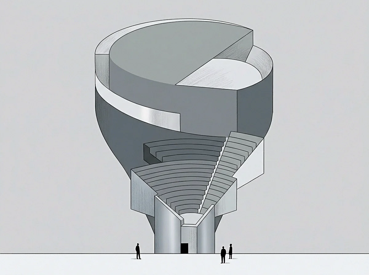
Shelf
A software architecture running a specialized machine learning pipeline at a seventy thousand dollar monthly operational loss reveals a clear gap between projection and physical reality. Engineering leadership projects forty million transactions per hour based on component specifications, but operational logs show the deployment pipeline continuously routing data around the central optimization engine to cap real throughput at four million transactions. The system pays for the full compute cluster while actively using only a fraction of its capacity.
This variance between projected output and what a system actively avoids producing marks an epistemic gap. Projected capacity models rely on cardinal arithmetic derived from theoretical ceilings, whereas observed behavior follows an ordinal vector shaped by operational friction. Forcing high-volume workloads into these avoided paths degrades performance rapidly or triggers unhandled timeout cascades.
System avoidance vectors mark the precise coordinates where operational computation becomes prohibitively expensive.
Avoidance reflects direction rather than an operational defect. The system steers work away from specific pathways because those routes incur high execution times, memory overhead, or state lock contention. An operator watching this shift often mistakes it for a training deficiency or configuration error, but the mechanism is purely mechanical: the architecture takes the path of least resistance across its state space to maintain stability.
Capital spent expanding cluster allocations under the assumption of latent throughput yields no return while the avoidance vector remains unaddressed. Infrastructure expenses escalate as the operational footprint contracts toward its baseline. Price is a single figure, whereas cost operates as an ordinal vector; confounding the two leaves performance capacity models detached from physical runtime realities.
Treating an avoidance vector as a simple performance failure instead of a structural coordinate leads directly to wasted capital on unviable capacity expansions.

Slope
The trajectory an architecture follows through its state space always conforms to the path of minimal energy expenditure. Every computational environment defines a value axis across its operations, where the derivative of movement yields a mathematical gradient that measures the rate of change in execution cost across adjacent system states.

Can Unspent Capacity Exist Without An Avoidance Vector?
Projected latent capacity is a mathematical reflection of a system’s avoidance pattern. When an operational boundary keeps a system out of a specific processing domain, the unspent capacity sits directly opposite that boundary across the baseline. The magnitude of the avoidance vector equals that of the latent capacity volume, making them inseparable in system analysis.
- The local minimum defines the state configuration where small parametric shifts in any direction increase immediate operational friction, locking system movement in place.
- The ascent gradient measures the exact computational energy input needed to move system state away from its path of least resistance toward high-throughput configurations.
- The baseline reflection maps the theoretical volume of unspent processing potential by projecting the inverted magnitude of observed avoidance coordinates above the current performance baseline.
The system routes around the peak. Trying to climb the ascent gradient without modifying underlying structural constraints requires constant energy injection. The moment forced effort drops, the system slides back down the slope into its low-resistance minimum, returning automatically to equilibrium.
Latent potential mirrors the inverse magnitude of observed avoidance across the operational baseline when execution parameters remain constant.
Mapping this movement requires establishing a fixed temporal window. Operators who calculate gradients over isolated three-minute windows observe noise rather than direction, whereas evaluating movement across a forty-day window reveals the true baseline, fixing the scale and clarifying whether avoidance stems from transient spikes or structural limits.
An explicit terminal clause in the capacity SLA changes the system’s baseline evaluation from projected volume to verified throughput.
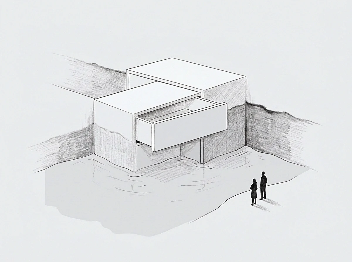
Ledge
Financial models frequently construct throughput expectations from theoretical component limits rather than empirical execution paths. Board reports and strategic plans often record projected capacity as an asset, ignoring the friction that prevents that capacity from converting into output. Comparing observed avoidance vectors against projected capacity metrics reveals the variance distorting operational forecasts.
| Operational Parameter | Observed Avoidance Vector | Projected Latent Capacity Volume | Epistemic Divergence Mechanism |
|---|---|---|---|
| State Synchronization | Routing around multi-region locks | Multi-region concurrent throughput | Serial execution constraints treated as temporary network latency |
| Data Pipeline Ingestion | Dropping complex schema transformations | Real-time unified schema analytics | Validation cost excluded from pipeline processing models |
| Resource Allocation | Throttling worker node creation | Linear elastic auto-scaling | State initialization overhead capping node provisioning speed |
| Data compiled from continuous architectural trace logs over a ninety-day evaluation window. | |||
The comparison illustrates that projected capacity figures routinely assume frictionless state transitions. In real infrastructure, validation steps, consensus checks, and memory garbage collection impose heavy penalties, prompting the architecture to redirect execution thread pools into simpler subroutines that register the real price.
Projected throughput derived without accounting for validation overhead represents speculative volume rather than usable capacity.
When leadership evaluates a system purely on projected capacity volume, structural avoidance vectors are forced underground. Operators introduce custom bypass scripts, soft validation limits, or unmonitored queues to simulate capacity utilization. The system appears to make progress, but structural debt accumulates silently at the boundary until a major state collapse occurs.
The infrastructure was allocated for twelve thousand concurrent tasks, yet the production configuration throttles at four hundred to prevent state corruption.

Gate
Computational systems hit hard operational boundaries whenever execution transitions from cached pattern retrieval to live state synthesis. Retrieval costs very little compared to live computation; within its cached domain, response times stay low and resource consumption remains flat. The moment workloads demand real-time state synthesis across distributed nodes, execution hits the wall.
The wall marks the boundary of a system’s current architectural model. Signals in operational monitoring systems—elevated CPU temperatures, queue depth spikes, and thread pool exhaustion—serve as exact instruments measuring computational density rather than failure. Systems operating at the wall perform actual computation instead of retrieving historical execution patterns.
Operational friction at the system boundary indicates active computation replacing static pattern retrieval.
Avoidance marks the coordinate where the current model stops functioning efficiently. Pushing past that coordinate without altering the underlying algorithm forces inefficient fallbacks, causing the system to route around expensive computation by returning default payloads, dropping optional metrics, or rejecting late-arriving requests.
It remains unresolved whether this structural boundary can be shifted through iterative parameter adjustments or if total re-platforming provides the only path past the current operational ceiling.

Trench
Reconciling the variance between actual output and theoretical ceilings demands an ordinal mapping of operational costs. Operators who stabilize high-throughput environments abandon cardinal capacity projections entirely, focusing instead on adjusting the physical gradient through structural modifications to the processing pipeline.
- Identify every execution path where processing threads routinely redirect workloads to secondary queues.
- Log the precise state lock duration and memory allocation cost associated with rejected execution paths.
- Re-index resource allocation based on observed ordinal friction rather than component throughput specifications.
- Mirror verified avoidance vectors across the operational baseline to determine true limits on unspent potential.
- Establish hard operational terms that restrict incoming workload arrival rates to verified throughput capacity.
Aligning incoming load with verified execution pathways sets a firm term, eliminating the cascading failures associated with forced capacity scaling. The system operates within its calculated low-friction domain while engineering teams systematically dismantle structural friction points along the wall.
Because computation costs energy, systems consistently seek a low-energy state space regardless of executive projections. Mapping the avoidance vector delivers the actual coordinates of system behavior, establishing a reliable foundation for long-term architectural stability.