
Determining Calibration Delays Across Capital Allocations When Operational Signals Fall Below Minimum Thresholds
A calibration delay balances statistical confidence against capital burn to prevent volatile operational noise from triggering disruptive capital adjustments.

Valve
Capital stays inside an operational channel until a metric breaches its floor. If an allocation running forty thousand dollars a month into customer acquisition shows three consecutive weeks of dropping conversion efficiency, the delta between baseline yield and realized volume can widen past thirty percent. Pulling capital immediately risks cutting off a recovery taking shape in downstream retention, while adding funds too early subsidizes broken mechanics.
The calibration delay marks the span between a recorded signal breach and the practical adjustment of funds. While operators often treat this period as administrative lag, it acts as a statistical filter to separate temporary variance from permanent degradation. Choosing this duration requires balancing the observation window directly against the signal’s half-life.
A rapid intervention converts statistical noise into organizational friction.
Signal volatility sets the minimum observation window. High-frequency metrics like paid click efficiency generate hourly noise that takes fourteen days to settle, while low-frequency indicators like enterprise contract expansion need ninety days to produce a single reliable delta. Cutting the delay shorter than the signal half-life leaves capital chasing false trends.
Letting it run past two signal cycles allows structural capital destruction to compound unchecked.
The interaction between capital velocity and threshold depth shapes the operational risk surface. A shallow threshold breached across a short window triggers repeated false reallocations, consuming administrative capacity and breaking operational momentum.

Drift
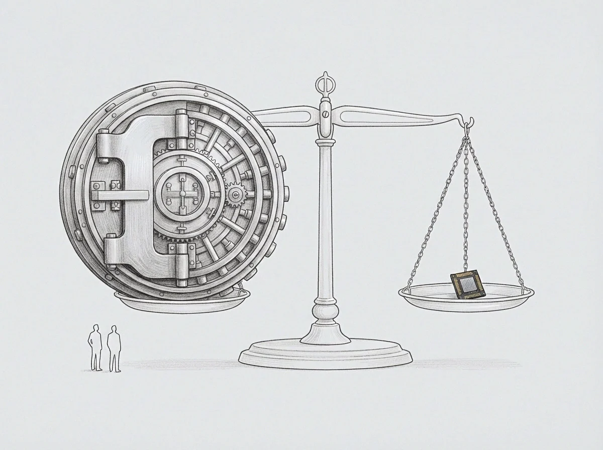
Observation Windows Across Operational Metrics
Different operational channels run at metric frequencies that cannot share a single review calendar. Engineering throughput shifts on two-week sprint cadences, while customer lifetime value updates across rolling quarters. Applying identical calibration delays to both produces asymmetric diagnostic errors.
Fast channels show acute drops right away, whereas slow channels gather deficits quietly until capital reserves run thin. An allocator sets an independent measurement window for each channel before deploying funds.
Intervention delays match the time required for a metric to register its true mean.
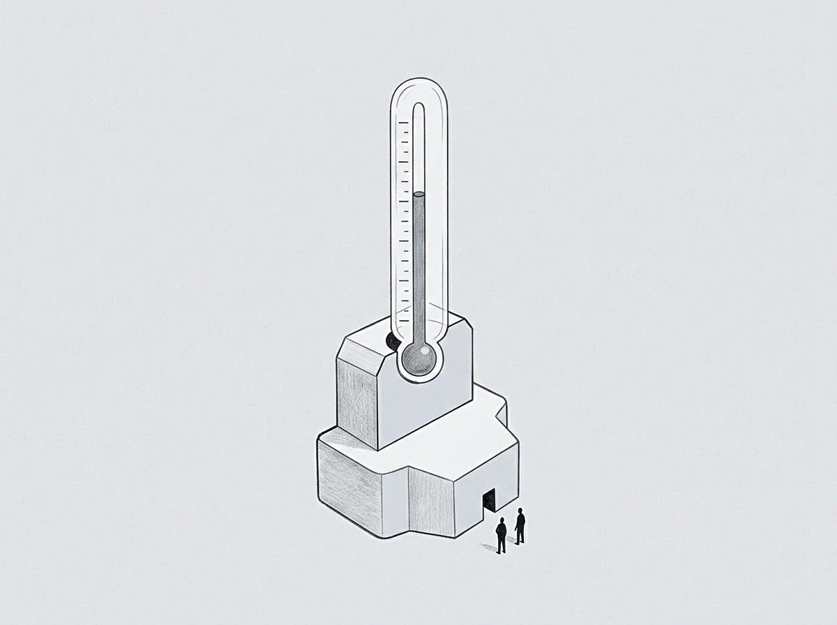
Structural Sources of Measurement Error
Operational signals drop below baseline thresholds through distinct failure modes that require different responses.
- Transient variance shocks occur when market turbulence or local operational hitches suppress yields without damaging the underlying conversion architecture.
- Permanent capacity decay happens when the addressable audience exhausts or production pipelines suffer irreversible unit economic degradation.
- Telemetry instrumentation flaws create false deficits through broken tracking pipelines, corrupted attribution scripts, or delayed database synchronizations that distort transaction counts.
Separating transient variance from capacity decay relies on covariance tracking. If paid acquisition drops while blended organic search conversions stay steady, external channel pricing is the driver. If organic conversion and paid efficiency fall together, the underlying conversion asset has decayed.
Isolating external macroeconomic shifts from internal asset decay during a liquidity contraction remains difficult for an operating team to manage in practice.
Rig
What Halts Capital Rebalancing Across Breached Allocations?
Automatic rebalancing pauses when signal confidence intervals exceed the expected return spread between allocations. Shifting capital from a depressed channel into an adjacent project introduces immediate friction and ramp delays. An allocator needs empirical confirmation that the breached channel yields less than the alternative once migration costs are factored in.
Signal confidence builds over time as each extra observation day reduces the standard error of the measured yield. The delay period marks the point where the cost of additional precision matches the capital burn of holding a sub-threshold position.
A capital pause holds until migration friction falls below the projected yield differential.
| Signal Type | Variance Profile | Minimum Threshold Deficit | Optimal Calibration Delay | Capital Rebalancing Action |
|---|---|---|---|---|
| Paid Acquisition CAC | High Daily Dispersion | 20 Percent Yield Drop | 14 Calendar Days | Taper Tranches by Half |
| Enterprise Sales Pipeline | Low Frequency Clumping | 35 Percent Pipeline Dip | 60 Calendar Days | Freeze Territory Expansion |
| Platform Infrastructure Unit Cost | Deterministic Step Functions | 15 Percent Gross Margin Loss | 7 Calendar Days | Route Traffic to Baseline |
| Subscription Cohort Retention | Slow Multi-Month Decay | 10 Percent Renewal Contraction | 90 Calendar Days | Quarantine New Commitments |
The Mechanism of Window Selection
Setting a delay window balances sample size against the rate of capital depletion. Allocators evaluate the cumulative cash exposed across the observation window; a channel spending five thousand dollars per day allows for a longer test than one spending fifty thousand dollars per day under the same cash constraints.
The capital allocation rules pause funding automatically once cumulative threshold deficits exceed fifteen percent of the total quarterly channel budget.

Tier
Dynamic Adjustment of Threshold Boundaries
Static thresholds fail in shifting market environments. If industry-wide conversion rates drop ten percent from seasonal contraction, a fixed threshold can trigger an unneeded capital freeze. Dynamic boundaries account for this by indexing internal performance to broader sector trends.
Dynamic bands still require hard floor parameters so relative indexation does not mask absolute losses. An operating model requires positive cash generation regardless of how competitors perform.
Stepwise Capital Calibration Sequence
- Signal validation scan verifies raw data pipelines to eliminate reporting errors before manual review begins.
- Threshold deficit quantification calculates the variance spread between the target baseline and the observed thirty-day rolling average.
- Delay clock initiation starts a fixed observation window with frozen operating parameters to collect clean variance data.
- Tranche adjustment execution steps down capital transfers in increments rather than making full withdrawals, preserving room for operational recovery.
When an automated drawdown triggers after a signal breach, the operating team works on operational execution rather than disputing the underlying rule.
A temporary signal drop often reflects pipeline fluctuations that normalize before the calibration window closes.
Trace
Decoupling Capital Ramps From Cached Assumptions
Allocators often lean on historical baselines formed under outdated conditions. When broader economic conditions shift, older assumptions delay the recognition of real performance deficits. Tracking live metrics requires steady updates to expected return distributions.
Quick decisions often hide a reliance on static reference points. Making an allocation change minutes after a signal breach usually draws on past patterns rather than real-time statistical evaluation, which requires measuring the exact spread between present performance and baseline targets.
Uncalibrated delay extensions convert temporary operating deficits into permanent balance sheet liabilities.
Executing Post-Threshold Reconstitution
Restoring capital to a recovering channel requires evidence that holds across an entire evaluation cycle. One week of performance above the threshold does not prove recovery after a prolonged slump. The recovery window matches the calibration delay to provide balanced statistical confidence.
Funding returns in stages aligned with historical throughput. If the channel holds baseline yields across two full observation cycles, allocations return to initial target levels. The process ends once operational telemetry stabilizes at baseline under full capital load.