
Determining Optimal Observation Window Durations Before Declining Directional Delta Triggers Complete Operational Reallocation
An observation window matches the signal noise period to verify directional decline before operational reallocation shifts active capital.

Gate
A software project logged ninety days of consecutive net cash deficit while daily operational throughput climbed by fourteen percent. Financial accounts recorded steady losses, but performance indicators showed clear upward momentum across primary production channels. Decision makers evaluated whether to liquidate the asset or maintain funding.
Pulling capital from an active channel during a contraction often destroys value when underlying metrics reflect transient turbulence rather than fundamental failure.
Separating random variance from structural decline requires a fixed observational timeline before making operational adjustments. Intervening early risks mistaking statistical noise for terminal decay. Operators who alter resource allocations too quickly cycle through strategy changes without accumulating actionable data.
A structured evaluation period binds executive action to quantitative changes rather than immediate reactions to temporary downturns.

Initial Measurement Principles
Establishing baseline metrics requires historical stability before tracking active performance trajectory. An operational shift can only be identified against documented standard values, as the initial monitoring phase defines the expected variance during normal production. Without that baseline, ordinary operational fluctuations read as systemic errors.
- Baseline Calibration establishes the fixed reference point from thirty days of static activity before measuring any trajectory shift.
- Directional Delta measures the ordinal trajectory of performance movement rather than isolated absolute numbers.
- Observation Window fixes the minimum elapsed time required to separate random variance from true system decay.
Every operational process exhibits natural variation. Production velocity speeds up and slows down based on external market inputs and internal processing limits, and a transient drop does not indicate systemic breakdown.
An observation window lasting fewer than three operational cycles misinterprets stochastic volatility as systemic decline.
When tracking performance trajectories across consecutive operational periods, a drop exceeding two standard deviations over a fixed forty-five-day evaluation window triggers a mandatory review of channel asset distribution.

Threshold
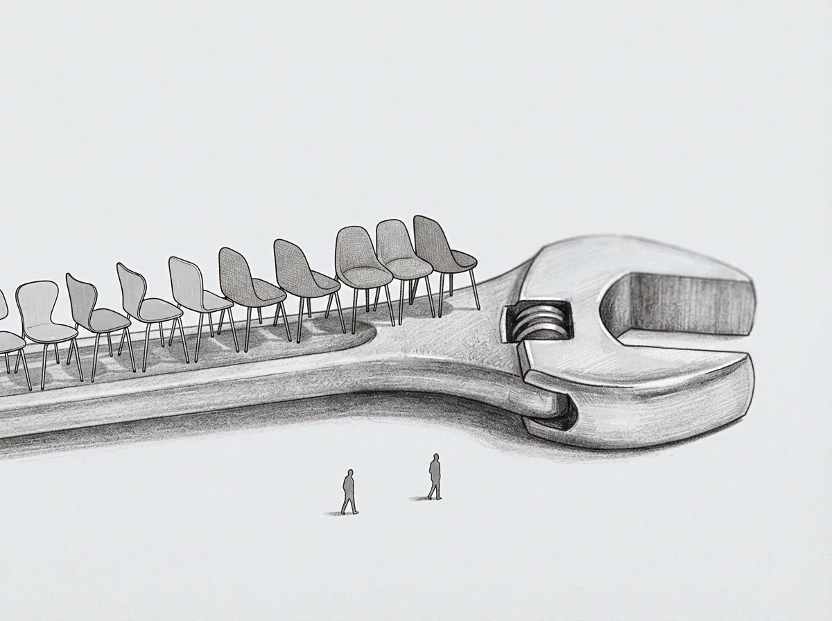
Operational scale dictates the required length of a monitoring period. High-frequency consumer transactions yield immediate statistical feedback, whereas enterprise software deployment cycles require months to show meaningful trend lines. Matching evaluation lengths to the underlying operational frequency prevents premature capital migration.
Setting evaluation boundaries requires balancing transaction costs against channel degradation risks. Short observation periods limit financial exposure to failing operations but increase reallocation overhead. Longer periods protect ongoing projects from temporary disruptions while risking sustained capital waste on dying initiatives.
Variance Across Operational Scales
Determining timeline parameters involves categorizing organizational functions by asset turnover rates and feedback lag. Fast feedback loops require compact evaluation timelines, whereas extended projects require enough time for compounding inputs to show measurable movement.
| Operational Level | Minimum Window Duration | Signal-to-Noise Ratio | Reallocation Trigger Delta |
|---|---|---|---|
| Micro-operations | 14 Days | 4 to 1 | 15 Percent Sustained Drop |
| Cohort Operations | 90 Days | 2 to 1 | 22 Percent Sustained Drop |
| Asset Allocation | 180 Days | 1 to 1 | 30 Percent Sustained Drop |
An improper evaluation duration distorts performance signals. A team monitoring daily conversions over a forty-eight-hour window mistakes routine weekend volume dips for structural failure. Conversely, tracking annual enterprise account expansions with multi-year metrics delays corrective shifts long after customer retention collapses.
A minimum window of ninety days prevents temporary quarterly compression from liquidating long-term assets.
Reallocating assets based on incomplete observational periods incurs systemic transaction expenses that routinely exceed the operational losses recorded during the evaluation period itself.

Gradient
Calculating the rate of decline provides clearer analytical signal than recording static losses alone. A negative trajectory that stabilizes at a lower equilibrium demands a different operational response than an accelerating downward slope, and tracking derivative movement over time exposes the true rate of channel decay.
Assume two business units each experience a twenty percent reduction in active monthly revenue. The first unit experiences a flat five percent drop every week for four consecutive weeks. The second unit drops eighteen percent in week one, then stabilizes with less than one percent weekly variation over the remaining three weeks.
The overall drop matches, but the underlying mechanisms differ fundamentally.

What Alters the Speed of Resource Reallocation?
Evaluating decay rates requires testing system responses against dynamic environmental inputs. Static decision algorithms execute cached responses instantly upon reaching arbitrary loss limits, whereas dynamic evaluation processes calculate the continuous rate of change across multiple successive observation windows.
A continuous decline across consecutive windows signals structural asset decay. When the derivative of the delta stays negative over two full tracking cycles, active capital transfers to higher-performing operational channels. The operator shifts resources only when trend line stability confirms continuous deterioration.
Reallocation executed before the window completes converts temporary operational noise into permanent asset losses.
A drop that halts before breaching the threshold indicates the establishment of a new operational baseline rather than terminal channel collapse.

Interval
Executing an operational shift requires a sequential protocol to prevent operational dislocation. Resource reallocation destabilizes teams and introduces administrative friction, which structured transition schedules help minimize during transfers.
The founder observes performance metrics through standardized reporting interfaces. Premature intervention compromises the observation window, introducing observer bias into the active dataset, whereas orderly execution protects historical data accuracy.

Execution Protocol for Operational Shifts
Moving resources between operational divisions follows a strict linear sequence to preserve tracking accuracy and operational continuity.
- Record sixty consecutive daily data points to calculate the operational median baseline.
- Track the directional delta across three full observation windows without modifying active assets.
- Reallocate capital only when the negative delta persists beyond the pre-established temporal limit.
Disciplined execution prevents subjective sentiment from overriding established statistical parameters. When performance metrics break lower limits consistently, operational changes proceed according to the predetermined transition schedule.
The original asset allocation remains entirely binding until the final observational boundary expires in full.
Decay
Extending observational windows indefinitely presents serious structural hazards to organizational solvency. Teams experiencing declining operational deltas frequently petition for longer evaluation periods to delay resource reallocation, shielding non-viable initiatives from necessary liquidations.
Continuous monitoring without clear reallocation boundaries generates severe administrative friction. Capital remains locked in stagnant operational channels while growth opportunities pass elsewhere, making rigid adherence to sunset schedules essential for operational flexibility.
Systemic Vulnerabilities in Extended Tracking
Organizational inertia routinely distorts window durations when projects underperform established benchmarks. Teams alter operational metrics mid-cycle to create the illusion of positive momentum, which objective evaluation procedures prevent by eliminating arbitrary timeline extensions.
A founder who continuously extends tracking deadlines absorbs mounting opportunity costs while protecting failing initiatives from capital redeployment. Clear analytical rules enforce reallocation decisions regardless of internal organizational pressure.
Operators routinely lengthen tracking periods when metrics drop to avoid executing uncomfortable asset shifts.
What structural modifications occur within an operational division when performance deltas remain stagnant just above the reallocation threshold for extended periods?