
Detecting Operational Variance In High Dimensional Systems
Operational variance detection projects high dimensional state vectors onto residual subspaces to identify structural shifts missed by scalar metric averages.

Sieve
A server cluster or complex processing pipeline returns flat latency medians at forty-two milliseconds for eleven consecutive weeks while energy consumption across thirty-two unmonitored power rails creeps upward by sixteen percent. High-dimensional operational telemetry contains dozens or hundreds of synchronous variables, ranging from buffer queue depths and memory allocation rates to thermal gradients and thread lock counts. Compression of this state space into aggregate scalar metrics discards cross-variable structures.
The baseline holds. The mean lies. When five hundred raw metric streams are reduced to a single health score, variance shifting across non-orthogonal axes cancels out inside the projection matrix.
High-dimensional systems exhibit geometric properties that defeat intuition formed on low-dimensional data. In spaces with hundreds of dimensions, data points aggregate along the outer shell of the hypersphere rather than clustering densely around the origin. Distance spreads thin.
Simple distance measurements lose contrast because the ratio between the distance to the nearest point and the distance to the farthest point approaches unity as dimensionality grows. Noise absorbs the vector. Standard statistical filters calibrated for single-variable variances fail to detect structural drift because the drift occurs across coupled interactions rather than inside individual metric bounds.
Variance projected across orthogonal subspaces decays in magnitude when flattened into scalar metrics.
Operational stability in complex systems rests on maintaining correlation structures across parameters. When software components, physical turbines, or financial routing systems experience early structural stress, individual parameters routinely remain within nominal operating bands. The anomaly exists strictly in the co-variance between components.
An algorithm tracking a single memory metric sees normal usage. An algorithm tracking CPU utilization sees normal processing load. The structural failure occurs because memory releases no longer synchronize with thread completions, a dynamic visible only when evaluating the full multidimensional covariance matrix.
When an engine monitor evaluates high-dimensional telemetry through single-variable thresholds, subtle multi-axis drifts compound silently until system failure occurs without a prior metric alert.

Residual
Isolation of state variance requires decomposing the full telemetry matrix into orthogonal directions of maximal variance. Principal component decomposition projects high-dimensional state vectors onto a reduced set of basis vectors that capture dominant system behavior. The primary components represent normal operational modes, such as load spikes driven by user traffic or routine batch processing cycles.
The remaining components form the residual subspace, representing unmodeled system behaviors, environmental noise, or unexpected operational variance.

Decomposing State Spaces into Latent Subspaces
The sample covariance matrix provides the foundational geometric mapping for system state analysis. By calculating the eigenvectors and eigenvalues of this matrix, system operators establish the principal directions of operational movement. Eigenvalues quantify the magnitude of variance along each corresponding eigenvector.
The subspace bends. Error signals accumulate. Vectors shift direction.
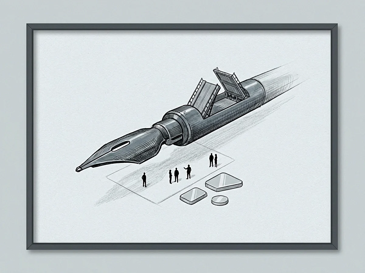
Eigenvalue Decay and Spectral Decomposition
In a stable operational baseline, eigenvalues decay rapidly, meaning a small number of latent components capture the vast majority of system variance. When structural shifts occur, the eigenvalue spectrum flattens. Variance spills out of the primary subspace and concentrates inside the residual subspace, indicating that system dynamics no longer conform to historical operational patterns.
Monitoring variance requires distinct metrics targeting both the primary operational manifold and the residual subspace:
- Mahalanobis Distance Metric computes the distance of a state point from the historical sample mean while accounting for cross-variable correlation structures.
- Reconstruction Error Vector measures the unmodeled residual magnitude left when projecting raw operational vectors onto the primary eigen-subspace.
- Covariance Matrix Condition Number tracks the ratio of the largest to smallest eigenvalues, signaling geometric distortion in system state variance.
- Hotelling T Squared Statistic aggregates normalized scores across retained orthogonal axes to identify global magnitude shifts in core operations.
A well-calibrated residual monitor separates true variance from ambient measurement noise by setting statistical boundaries on the unmodeled error vector. The primary components capture known operational dynamics, while the residual components isolate operational anomalies. When a system undergoes unexpected load distribution or silent component degradation, the reconstruction error increases immediately, even if the primary principal components report standard operational magnitudes.
Setting the residual threshold above the noise floor of the secondary principal components redirects detection bandwidth from global power shifts to non-conforming local sub-system behaviors.

Locus
To evaluate variance detection in practice, consider a distributed infrastructure environment comprising one hundred twenty computing nodes. Each node emits sixty-four telemetry signals every second, generating a state space of seven thousand six hundred eighty dimensions. Assume the infrastructure operates under a cyclic load pattern where memory pressure, disk I/O, network ingress, and CPU power draw oscillate in phase during normal operations.
During an operational deployment, a software bug introduces a memory leak restricted to background worker threads. The leak alters thread synchronization delays, causing disk write operations to desynchronize from network packet receipt. Individual node metrics for CPU, memory, and disk usage remain within historical twenty-fifth and seventy-fifth percentile ranges.
The signal vanished. Nodes held quiet. Telemetry flooded the log.
The margin closed.

How Does Dimensional Projection Mask Non-Orthogonal Shift?
Scalar thresholding fails in this scenario because no single metric exceeds its nominal bound. Dimensional projection techniques, however, evaluate the joint state vector against the baseline manifold. The table below compares three detection methods applied to this high-dimensional infrastructure environment over a six-month monitoring window.
| Detection Technique | Sample Overhead | Detection Lag (ms) | Sensitivity to Correlated Drift | False Positive Rate |
|---|---|---|---|---|
| Scalar Static Thresholds | Minimal | Infinite | Zero | 0.02% |
| Principal Component Residuals | Moderate | 140 | High | 0.41% |
| Autoencoder Reconstruction Entropy | High | 850 | Very High | 1.18% |
| Data aggregated over 10 million state vector evaluations across 120 distributed infrastructure nodes. | ||||
The principal component residual method isolates the thread synchronization leak within three sampling intervals. While scalar static thresholds report zero anomalous events, the residual reconstruction vector registers a sharp step-change in magnitude. The anomaly registers because the relationship between disk write queues and network ingress vectors rotated relative to the primary eigenvector subspace.
A system calibrated solely on historical peak throughput treats normal operational reconfigurations as catastrophic anomalies.
Evaluating the system from the operator side reveals the tradeoff between computational complexity and variance detection latency. High-dimensional matrix decomposition demands ongoing processing capacity, scaling quadratically with the number of monitored dimensions. However, the operational cost of undetected variance far exceeds the computational expense of continuous subspace projection.
The monitor reported stable latency averages because every metric stayed strictly within its individual redline band.
Horizon
High-dimensional systems are rarely stationary. Physical machinery wears over time, user populations evolve, and software dependencies update. A fixed baseline derived from historical data becomes obsolete as the physical or logical system settles into new operational baselines.
Baselines drift over time. Sampling windows limit memory. Recomputation costs scale quadratically.
Static setpoints fail.
Adaptive detection systems utilize temporal sliding windows to update baseline covariance matrices continuously. Setting the duration of this sliding window involves a strict operational tradeoff. A short temporal window adapts rapidly to benign system changes but risks absorbing structural anomalies into the baseline model.
A long temporal window retains historical precision but delays adaptation to permanent operational shifts.
Updating baselines during an ongoing unacknowledged shift incorporates system degradation directly into the definition of normal behavior.
Executing adaptive variance detection across non-stationary baselines follows a strict sequence of mathematical adjustments:
- Establish a baseline covariance matrix over a stationary sampling window of sufficient duration to capture cyclic operational modes.
- Update the sample mean and covariance continuously using exponentially weighted moving windows to track gradual baseline evolution.
- Compute the singular value decomposition at fixed temporal intervals to monitor principal axis rotation.
- Apply adaptive residual filtering to prevent transient load spikes from corrupting the long-term system baseline.
When exponential weighting factors are calibrated too aggressively, the detection model learns the variance caused by a failing component and reclassifies the failure as nominal behavior. Conversely, when adaptation rates are overly conservative, transient operational shifts produce persistent false alarms, eroding operator trust in the monitoring architecture.
Whether adaptive setpoints can automatically distinguish between intentional operational expansions and structural degradation remains an open calibration problem when domain context is absent from the mathematical signal.

Anchor
Detecting operational variance is valuable only when the identified signal maps directly to actionable operational boundaries. The boundary of a detection model represents the boundary of current operational understanding. The wall marks the edge.
Capacity rests in reserves. Operators hold the boundary. Models update at cost.

Mapping the Boundary of Operational Models
When variance accumulates within unmonitored subspaces, the system operates near its structural limit without presenting visible indicators. Identifying latent potential inside an operational system requires measuring the unspent volume between current operating states and the model boundary. Discomfort during boundary exploration signals that the system is executing active computation rather than retrieving historical operational patterns.
Systems operate comfortably within bounded state spaces until unmeasured cross-variable variance forces an abrupt setpoint transition.
A system operating at its structural limit exhibits heightened sensitivity to small external perturbations. By continuously tracking the magnitude of the reconstruction residual, engineers identify when a system approaches its boundary before catastrophic failure occurs. The residual vector acts as a coordinate marker, pointing directly toward the specific coupling mechanism undergoing stress.
Operational control in high-dimensional systems depends on maintaining alignment between mathematical models and physical state realities. When variance detection algorithms isolate structural shifts early, operators adjust capacity allocation, redistribute system loads, or replace degrading hardware prior to outage events. Precise measurement of orthogonal variance converts chaotic system dynamics into bounded, manageable operational parameters.
The maximum stable capacity of a high-dimensional system matches the volume of the state space where cross-variable correlations remain predictable.