
Extracting Clean Direction From Raw Spatial Performance Data
Spatial trajectory extraction isolates clean operational direction by subtracting environmental friction vectors from raw telemetry coordinates.
Grid
Positional tracking engines generate vast streams of spatial coordinates during standard automated runs. High-frequency sensors mounted on mobile equipment register latitude, longitude, elevation, and time. In ideal conditions without physical barriers or surface variance, these coordinate traces form straight lines from origin to destination.
Real operating environments present structural walls, terrain elevation changes, traffic congestion, and physical hazards, forcing assets to veer, stop, and detour around immediate impediments.
Spatial Telemetry and Surface Impedance
Automated tracking systems capture location coordinates every hundred milliseconds throughout an operational shift. Raw data displays erratic zigzagging patterns, velocity drops, and unexplained lateral excursions. Analysts examining unadjusted movement files frequently mistake defensive detours for intentional spatial shifts.
An asset steering thirty degrees off heading to avoid loose gravel on a haul road is executing surface avoidance rather than changing its target destination.
A recorded path reflects physical obstacles rather than pure destination intent.
Separating environmental impedance from primary motion requires a spatial reference baseline. Measuring the instantaneous spatial gradient along a trajectory reveals whether speed reductions stem from steep inclines or mechanical throttling. When a haul truck climbs a seven percent grade, kinetic reserve drops predictably according to gravitational mass calculations.
When speed drops along a flat corridor, operational friction or vehicle density accounts for the loss. Treating unadjusted spatial coordinates as direct intent forces the system to rebuild pathways around temporary obstructions, doubling transit time across the operational cycle.

Filter
Raw coordinate logs collect ambient noise from ground slipping, sensor drift, and structural detours. Filtering algorithms systematically isolate external friction vectors from the primary motion trajectory. A common approach applies discrete Kalman filtering to smooth sensor telemetry across low-density terrain, relying on Gaussian noise distribution assumptions in spatial telemetry logs across open operating zones.
Non-Gaussian multipath interference inside narrow metallic structures invalidates standard filter parameters, warping spatial estimates toward physical bulkheads.
Isolation of Environmental Resistance Vectors
Physical obstacles force moving equipment to diverge from straight spatial paths. Systemic divergence occurs in predictable patterns whenever spatial boundaries constrain transit options.
- Static Boundary Reflection occurs when an asset turns prematurely because a temporary barrier blocks the designated corridor.
- Local Minimum Trapping holds an autonomous unit inside a bounded loop while searching for immediate clearance.
- Lateral Drift Accumulation corrupts long-range tracking when steering adjustments stack without periodic recalibration against fixed survey benchmarks.
When an asset encounters a physical barrier, its directional response forms an acute avoidance angle relative to the obstruction surface. Measuring this avoidance coordinate identifies the perimeter wall of the spatial model. The magnitude of the lateral deflection matches the spatial resistance offered by the barrier.
Subtracting environmental resistance from raw positional tracks yields the true directional intent behind the path.

Slope
Physical elevation changes and operational friction alter movement velocity across spatial terrain. Calculating spatial direction requires evaluating the potential energy field surrounding the asset. Motion follows the line of least resistance unless driven by external kinetic inputs.
A vehicle moving across a contoured surface naturally descends along the steepest downward angle, converging on local floor depressions.

Gradient Derivation Across Variable Surfaces
Engineers calculate the change in potential energy across consecutive spatial sample intervals. Evaluating raw positioning against surface contours determines whether acceleration matches terrain geometry or reveals active driver steering. Comparing raw positional tracking against derived gradient calculations highlights key operational differences.
| Extraction Mode | Input Baseline | Impedance Handling | Vector Resolution | Operational Cost |
|---|---|---|---|---|
| Raw Positional Telemetry | Discrete coordinate pairs | Ignored or averaged | Superficial heading | Low initial processing |
| Derived Gradient Trajectory | Continuous potential surface | Explicitly isolated | True directional axis | Higher computational density |
| Derived gradient trajectories isolate intent by removing surface friction from raw positional logs. | ||||
Ascent costs kinetic reserve. A vehicle climbing a steep grade burns unspent volume in its power cell to maintain forward momentum. Mirroring this negative ascent gradient above the terrain baseline reveals the latent potential of the vehicle trajectory.
When kinetic energy expenditure exceeds terrain gravity demands, the asset executes deliberate work against surface drag.
When spatial acceleration matches surface grade, the movement vector aligns with the underlying value axis.
The elevation threshold condition cancels recorded lateral deviations whenever the measured ascent cost exceeds the primary vector threshold.
Bearing
Directional alignment emerges after removing environmental detours from the accumulated positional record. The resulting directional vector, with magnitude scaling alongside effort, represents pure operational intent stripped of local evasive adjustments. Potential field navigation models project spatial movement options by assigning repulsive forces to known barriers and attractive forces to primary targets.
Continuous spatial gradient assumptions hold true in wide physical workspaces, but discrete step-function barriers break continuous gradient models at physical boundaries.
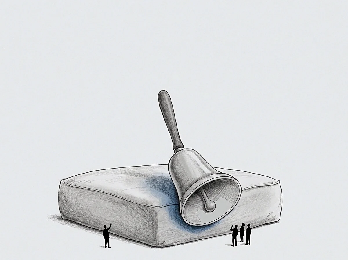
Does Uncorrected Movement Mask The True Goal?
Raw tracking logs frequently show assets steering far away from their assigned operational targets. A supervisor reviewing raw movement files might conclude that an operator abandoned the designated corridor entirely. Correcting raw logs for spatial friction demonstrates that the vehicle maintained maximum forward bias toward the goal while navigating around flooded terrain.
Spatial avoidance acts as an explicit coordinate marker for unmapped operational hazards.
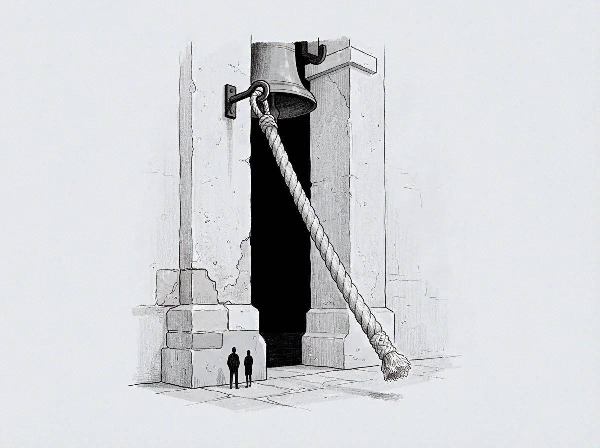
Sequential Vector Calculation Steps
Extracting pure motion targets demands a systematic numerical progression.
- Establish the reference baseline from stationary calibration benchmarks.
- Calculate instantaneous velocity vectors across consecutive sample windows.
- Compute local surface resistance forces from historical asset drag profiles.
- Subtract environmental impedance vectors from the observed velocity array.
- Project the resultant unconstrained directional vector onto the target spatial map.
A system routing around structural obstacles accumulates unprocessed spatial drag along its boundary wall.
The machinery followed the designated coordinates, but physical resistance forced the path to curve around the unmapped terrain.

Contour
Mapping the operational perimeter defines the boundaries where movement costs escalate steeply. Every spatial model contains boundaries beyond which asset propulsion becomes ineffective or inefficient. The physical wall represents the limit of active movement under current operational parameters.
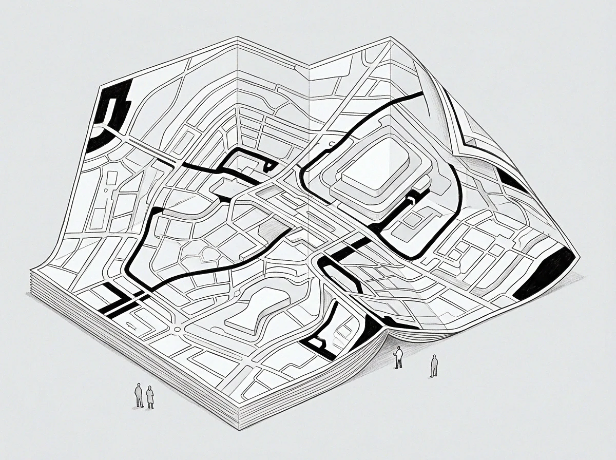
Boundaries of Spatial Potential
Unspent volume accumulates outside the active transit area, marking regions where operational friction halted forward progress. In industrial facilities, high equipment density creates tight spatial bottlenecks. Assets operating near these perimeters display rapid directional changes and high energy expenditure per meter advanced.
The exact threshold where human operator intervention overrides automated spatial steering remains unmeasured across dense industrial facilities. Under this uncertainty, an operator establishes conservative physical keep-out zones around dense machinery clusters. Mapping spatial contours isolates clean operational direction from raw telemetry, converting noisy movement traces into reliable navigational decisions.
The question remains whether unexpected spatial curvature reflects unmapped physical terrain or hidden human intervention.