
Establishing Calibration Protocols Across High Variance Real World Data Stream Windows
Dynamic multi-scale windowing stabilizes calibration by evaluating stream variance across stacked temporal partitions before updating baseline parameters.
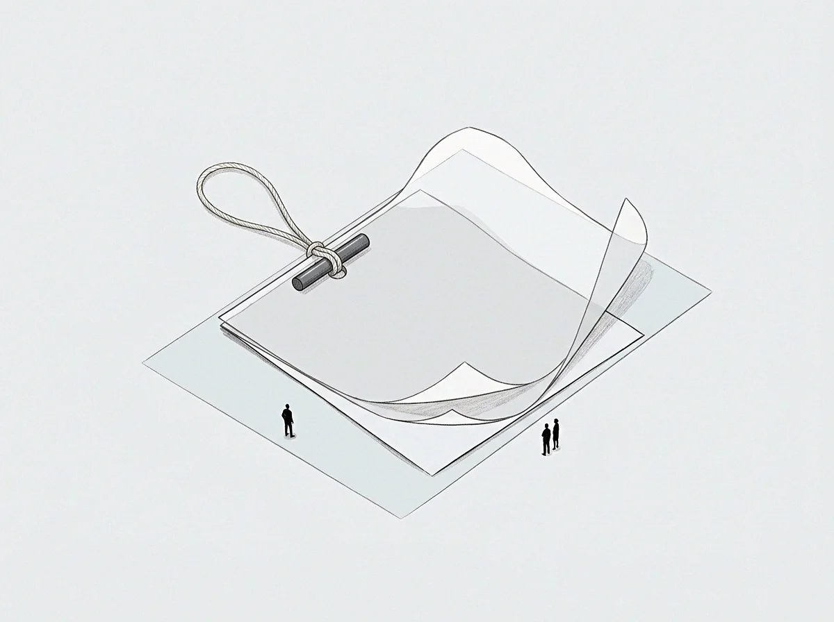
Shelf
Incoming data from physical production lines, transaction ledgers, and telemetry pipelines often shows sudden amplitude swings that destabilize static prediction boundaries. When an operational model ingests uncalibrated streams, raw variance corrupts downstream probability distributions within minutes. The person in the operational seat records the initial distribution on day one, setting an observation interval to watch how real event volume alters the feature space.
Without an empirical reference class, sudden fluctuations force reactive parameter edits that degrade long-term reliability.

Partitioning Real Time Ingestion Flows
Stream calibration separates volatile event noise from persistent statistical movement. A high-variance feed carries transient spikes caused by network latency, batch retries, or physical sensor interference. Ingestion pipelines buffer these events across a rolling partition, calculating the empirical cumulative distribution before any decision engine reads the output.
The baseline acts as the reference floor.
A rolling buffer converts raw event telemetry into an ordered distribution before parameter scoring begins.
Statistical properties of live streams shift across distinct operating regimes. A manufacturing line running high-volume night cycles produces tight error distributions, whereas day shifts introduce human operator variance that widens the interquartile range. The calibration architecture treats these intervals as separate operational states rather than a single continuous distribution.
Tracking the transition between regimes prevents false drift alerts and preserves analytical capacity for structural system failures.
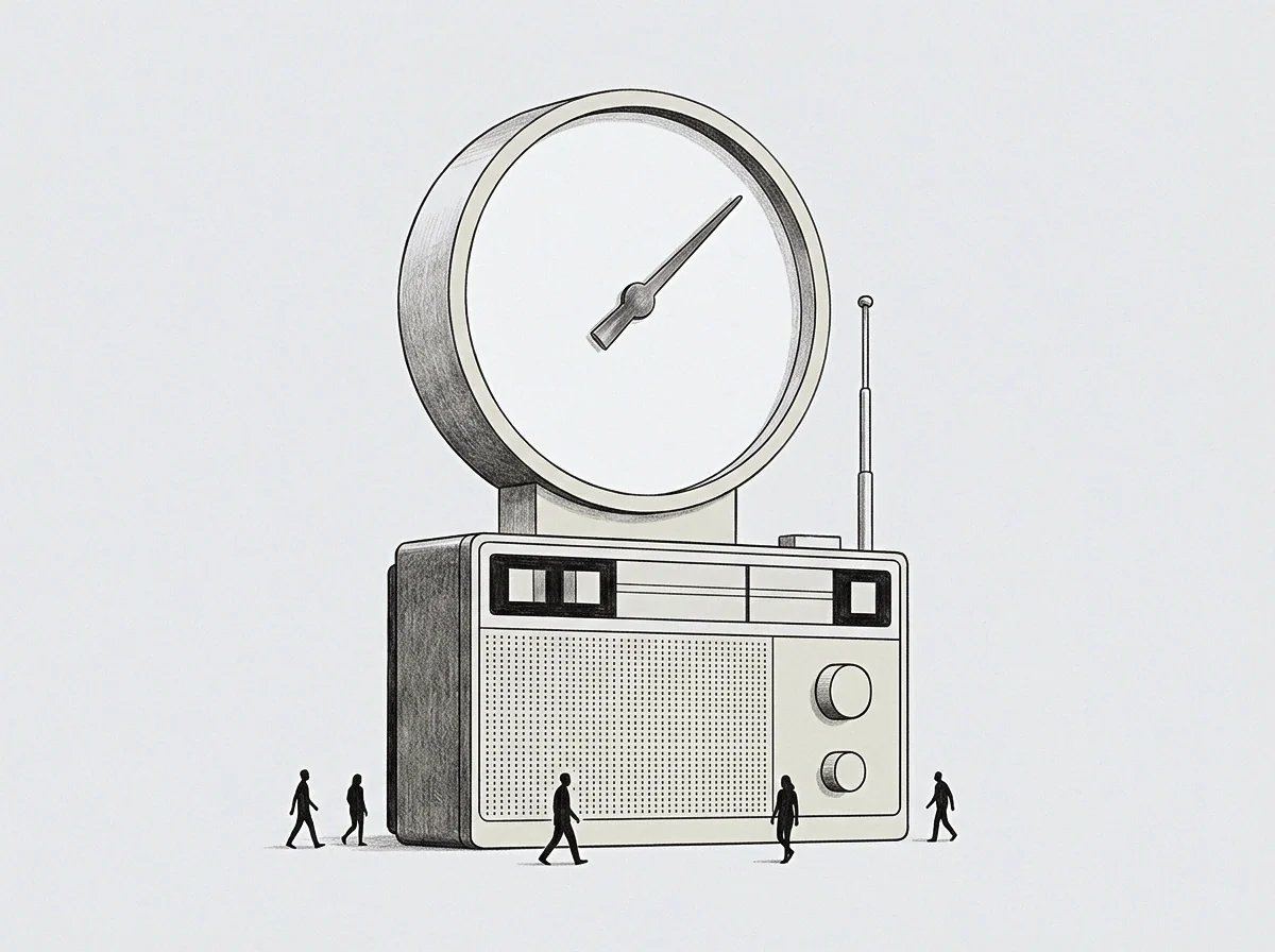
Spread
Dispersion across a live data stream points to either environmental volatility or structural degradation within the source process. Distinguishing between these states requires evaluating variance across multiple window scales simultaneously. A sudden expansion in variance across a ten-second window that dissolves across a ten-minute window constitutes transient turbulence.
Persistent expansion across consecutive hourly partitions signals a shift in the generating mechanism.
Variance Regimes in Non Stationary Streams
Evaluation pipelines measure dispersion using non-parametric order statistics rather than standard deviation. Extreme events skew linear dispersion metrics, causing calibration routines to overcorrect during temporary market or network shocks. The median absolute deviation provides an invariant baseline that resists outlier distortion while capturing systematic distribution widening.
- Interquartile Window Tracking isolates the central fifty percent of incoming observations across five-minute intervals to evaluate core stability.
- Ranked Order Quantiles monitor ninth-decile movement to detect tail expansion before mean shift becomes visible in aggregate logs.
- Median Absolute Deviation computes instantaneous dispersion relative to the rolling median, suppressing single-event outliers without dampening systemic trend detection.
Ignoring non-stationary dispersion leads to premature recalibration loops that bake transient anomalies into persistent operational baselines. When a system adjusts its scoring thresholds to accommodate brief volatility spikes, subsequent standard observations generate false negative alerts. The operator spends engineering hours diagnosing phantom sensor drift while real degradation accumulates unnoticed in the uncalibrated tail boundaries.

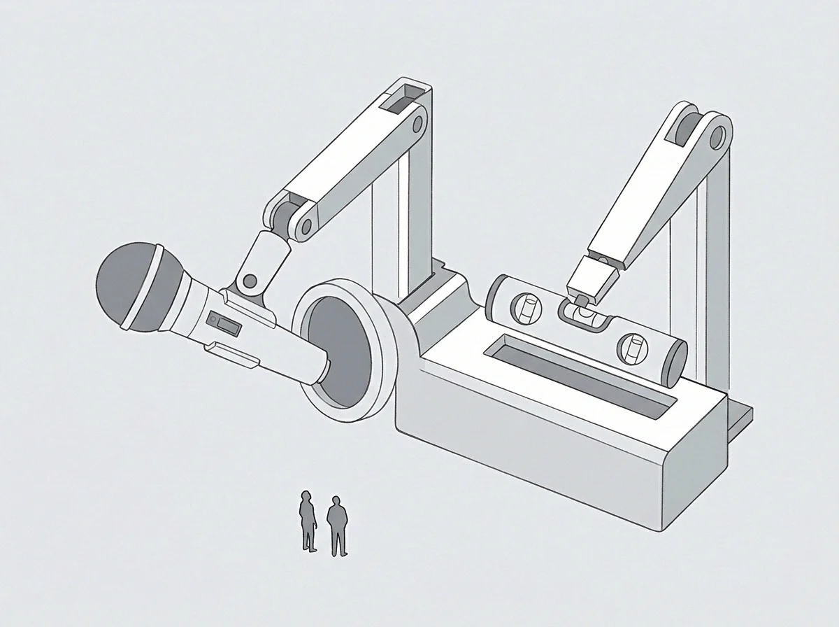
Band
Setting calibration boundaries requires defining explicit threshold bands that adjust to sustained input changes without tracking high-frequency noise. Static thresholds fail immediately in non-stationary production environments. Dynamic bands incorporate decay parameters that widen tolerances during known operational transitions and tighten bounds during steady-state processing.
| Calibration Strategy | Update Frequency | Computational Overhead | Outlier Sensitivity | Regime Shift Latency |
|---|---|---|---|---|
| Sliding Quantile Partition | Continuous per observation | High memory allocation | Low when using order statistics | Immediate adaptation |
| Exponential Decay Smoothing | Discrete time interval | Minimal compute cycles | Moderate under extreme shocks | Proportional to half-life setting |
| Adaptive Cumulative Sum Band | Event-triggered threshold cross | Bounded storage requirement | Very low via filtered buffers | Fast on persistent directional shift |
| Tumbling Batch Window | Fixed duration epoch | Low background processing | High within single partition | Delayed until epoch completion |

Boundary Adaptation Mechanics
The update rate of a threshold band governs its resistance to false alarms. Rapid adjustments track noise. Slow adjustments miss regime shifts.
Calculating the delta between short-term rolling variance and long-term historical spread reveals whether the input stream is experiencing temporary fluctuation or permanent structural realignment.
A calibration band tightens during steady observation and expands only when multi-window dispersion confirms persistent structural movement.
Calibrating probability outputs from classification systems demands continuous scaling against actual occurrence rates. Platt scaling and isotonic regression apply adjustments to static prediction scores, yet both methods deteriorate when incoming class prevalence shifts. In streaming environments, empirical binning over sliding time windows maintains alignment between model confidence and real outcome frequencies.
The baseline records the true positive rate across each quantile bucket.
A calibration threshold that moves on every observation destroys the reference class needed to interpret long-term drift.
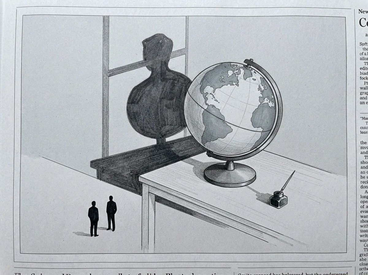
Cadence
Calibration intervals define the temporal resolution at which an operational system updates its internal scaling parameters. Selecting an arbitrary cadence introduces sampling bias that either conceals critical regime shifts or consumes unsustainable compute capacity. The sampling frequency aligns with the autocorrelation structure of the underlying data stream.

Does Real Time Recalibration Erase Trend Data?
Continuous adjustment updates baseline parameters on every arriving event. This high-frequency adaptation overwrites historical reference points, transforming slow, cumulative degradation into apparent stability. A sensor drifting one percent per hour appears calibrated if the window recalculates every sixty seconds.
The system erases the delta by integrating it into the baseline before the monitoring layer can register the error signal.
- Autocorrelation Extraction maps the temporal dependence length of the raw feed to prevent sampling within the noise horizon.
- Multi-Scale Window Stacking processes the stream through concurrent one-minute, one-hour and twenty-four-hour partitions to isolate immediate spikes from secular trends.
- Validation Trigger Checks compare live quantile distributions against the initial reference class, suspending automated parameter updates when divergence exceeds empirical noise ceilings.
What remains unresolved is the mathematical threshold at which automated systems can independently distinguish an engineered step-change in stream architecture from an unprecedented external macro shock.

Latch
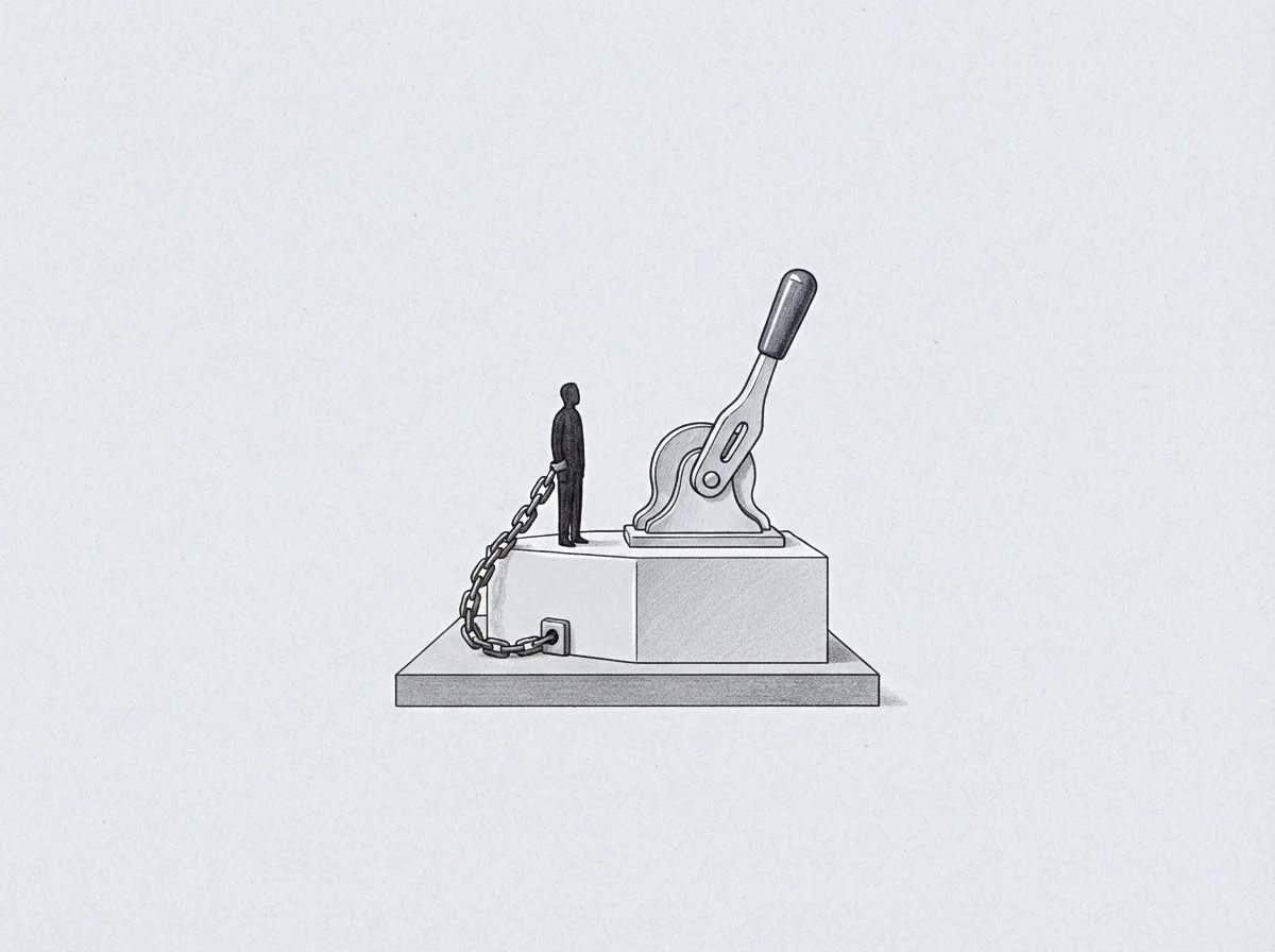
Preventing runaway parameter corruption requires a physical or algorithmic interlock that halts recalibration during catastrophic input corruption. The latch monitors stream integrity metrics independent of feature values. When input ingestion volumes drop below minimum density thresholds or missing-value rates exceed historical bounds, the latch freezes the active calibration parameters, forcing the system to fall back on conservative default baselines.
Execution of Automated Safeguards
Downstream systems require deterministic scaling guarantees. When upstream providers alter payload structures or timestamp formats, feature extractors produce corrupted zero-variance streams or erratic extreme values. An operational interlock detects structural corruption within milliseconds, isolating the corrupted feed and routing processing tasks to a cached fallback baseline.
An operational latch freezes baseline parameter updates the instant incoming data volume or structural integrity breaches empirical tolerances.
A structured data agreement specifies the exact allowable variance window, the maximum tolerated latency across stream partitions, and the fallback calibration state executed when incoming distributions breach acceptable bounds.