
Isolating Systemic Measurement Noise From True Directional Baseline Displacement
True directional baseline displacement alters physical resource constraints across multiple orthogonal axes while measurement noise remains localized to the recording pipeline.

Sieve

Sampling Cadence and Observation Artifacts
A daily dashboard metric swings eighteen percent across four consecutive mornings, even as total operating cash moves less than half a percent over the quarter. Watching the line oscillate, the operator adjusts server allocation, reorders deployment priorities, and drafts explanatory notes to capital partners. Three weeks later, the aggregate revenue curve sits precisely where simple linear extrapolation placed it before those adjustments began.
The daily fluctuations were artifacts of batch processing runs, payment clearing cutoffs, and client reporting cycles. Rapid shifts reflected the cadence of the recording apparatus rather than any change in customer demand.
Measurement noise enters observation pipelines through fixed periodicities, sensor precision limits, and aggregation delays. High-frequency variance regularly obscures low-frequency directional movement in an operational baseline. When an observer records an indicator over short intervals, noise from the recording tool often exceeds the underlying rate of change.
The baseline represents the true resting state of the operational system, whereas a directional displacement is a sustained shift in that resting state across a wider observation window.
A reading taken faster than the system completes its natural operating cycle records instrument volatility instead of true momentum.
Separating measurement artifacts from genuine momentum requires examining how telemetry actually aggregates data. When metrics aggregate at fixed hourly boundaries, that cutoff imposes artificial boundary conditions. Batch processing creates sudden surges, while weekend lulls lower reported volume.
These patterns repeat on predictable schedules, yet teams routinely mistake them for real expansions or contractions. Isolating true displacement starts by widening the observation window to swallow the full cycle of the measurement system.
Longer observation windows damp cyclical jitter. When the underlying baseline actually shifts, that displacement remains visible after regular operational cycles complete their turn.

Filter
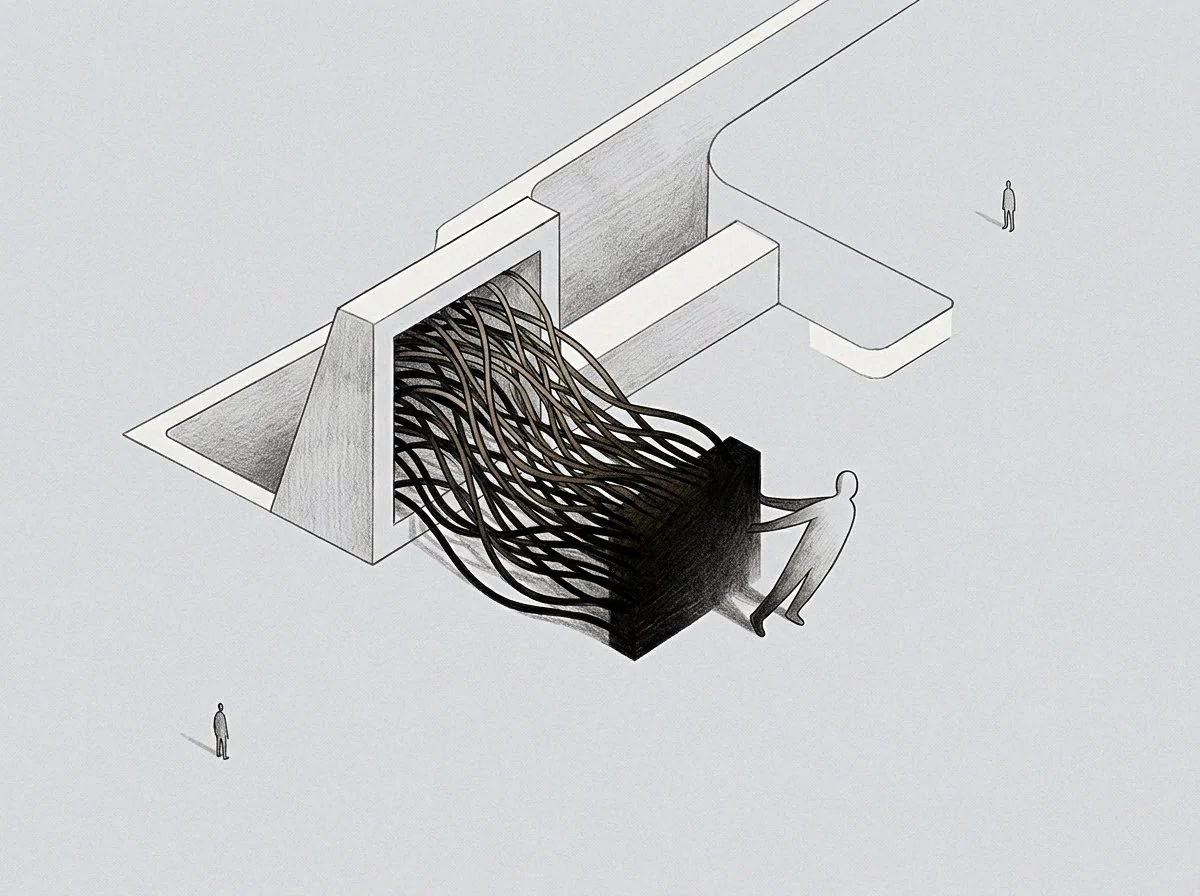
State Estimation Across Stated Windows
Distinguishing authentic displacement from observation jitter requires systematic state estimation. Direct observation yields a composite sequence containing both the true latent state and the disturbance introduced by data collection pipelines. Mathematical estimators separate these layers by weighting new data points against historical variance.
When noise is high, the model relies heavily on the historical trajectory, discounting single-period spikes. When noise is low and verified by physical counts, incoming readings quickly update the estimated state.
The table below compares three approaches to state separation across production data environments, evaluating their structural assumptions, computational latency, and vulnerability to false alarms.
| Separation Method | Primary Mechanism | Lag Profile | Vulnerability Mode |
|---|---|---|---|
| Moving Window Median | Rejects rank-order outliers within a fixed rolling temporal sequence | Fixed duration equal to half the configured sample period | Suppresses legitimate step-function shifts until the full window passes |
| Exponential State Estimator | Applies recursive fractional decay to historical observations | Low phase delay across continuous smooth transitions | Overreacts to sustained bursts of correlated observation noise |
| Orthogonal Component Decomposition | Isolates seasonal rhythms through frequency-domain spectral filtering | Variable latency dependent on multi-cycle data availability | Misattributes sudden structural baseline breaks to high-frequency harmonics |
Each method handles operational noise through different mathematical compromises. The moving median works best when dealing with isolated spikes, such as server timeout storms or payment gateway maintenance periods. An exponential state estimator tracks continuous trends with minimal computational overhead, though multi-day waves of noise can throw it off.
Spectral decomposition isolates predictable calendar noise with high precision, separating weekly payment cycles from underlying customer acquisition volume.
A genuine baseline displacement shifts the steady state of the system across multiple independent measurement axes at once. A marketing change that genuinely expands demand moves lead volume, qualification rates, pipeline velocity, and cash collection in a correlated sequence. In contrast, systemic measurement noise stays localized to specific collection nodes.
An instrumentation bug in a client script might inflate page views while pipeline velocity and server load remain completely flat. Cross-axis validation provides the definitive boundary check against sensor artifacts.
Mistaking localized sensor jitter for systemic growth leads directly to misallocated capital, premature hiring commitments, and liquidity shortages when unverified growth fails to materialize as real revenue.

Decay

Where Does Sensor Artifact Mimic Directional Movement?
Correlated noise mimics genuine structural displacement when disturbance terms fail to remain independent over time. In basic measurement theory, random noise possesses zero mean and cancels out across repeated observations. In commercial systems, however, measurement noise is frequently autocorrelated.
A change in data logging logic, a revised cookie consent banner, or a modified database index creates a permanent step in the recorded metric without altering real user activity by a single unit. The indicator shifts permanently, presenting the visual signature of a true baseline displacement.
Testing for invariance exposes the artificial nature of autocorrelated logging shifts. When a team encounters a sudden step-change in a tracked indicator, they run verification tests against independent physical artifacts:
- Resource consumption gradients track database input-output cycles, network egress volume, and power draw, confirming whether computational work grew alongside reported transactions.
- Secondary ledger reconciliation compares application logs against bank settlement statements and payment processor clearing files to verify that record counts match cardinal currency movements.
- Counter-metric equilibrium examines inverse operational indicators, verifying that customer support ticket volume, server latency, and inventory depletion reflect the scale of the recorded expansion.
Consider a practical operational situation. A SaaS business operating at eight hundred thousand dollars in annual run rate implements a revised telemetry pipeline on the first day of the second quarter. The primary activity dashboard immediately shows a forty percent surge in weekly active usage.
The product team celebrates the increase, attributing the jump to an interface redesign deployed forty-eight hours earlier. The operator, however, notes that server bandwidth remains unchanged at twelve gigabytes per hour, cloud hosting invoices show no computational expansion, and incoming support ticket volume stays at forty-two tickets per week.
A metric that leaps while its physical constraints remain undisturbed reveals an instrumentation shift rather than real organizational traction.
Tracing the telemetry event stream reveals that the new logging library counted automated background keep-alive pings as distinct user sessions. The forty percent increase in usage was pure instrumentation artifact. The true baseline had not displaced by even a single millimeter.
Had the organization scaled its infrastructure and expanded customer support based on the inflated user activity metric, operating margins would have collapsed under unneeded overhead.
The dashboard showed thirty thousand new users this month, prompting the team to scale support capacity before confirming real customer demand.
Anchor

Calibrating Directional Shift Across Resource Constraints
Establishing true baseline displacement demands physical grounding outside the digital reporting loop. Digital counters are cheap to increment and vulnerable to aggregation errors. Physical resources, cardinal currency exchanges, and human operating capacity carry strict constraints.
When true displacement occurs, it leaves an indelible footprint across these physical constraints. An organization cannot genuinely quadruple its client delivery volume without consuming additional employee hours, exhausting existing component inventory, or increasing gross banking settlements.
Reference class forecasting anchors the interpretation of directional movement. When an operator observes a claimed growth vector that exceeds the historical distribution of similar organizations within that sector, the burden of proof rests on physical confirmation. Calibration is the discipline of mapping internal confidence scores to empirical reality over extended time horizons.
The operator records a baseline on day one, defines a ninety-day observation window, and refuses to confirm directional movement until the window closes and physical reconciliation matches digital reporting.
Speed in declaring victory is almost always an artifact of cached assumptions. An organization that demands instant confirmation of strategic success inevitably mistakes the crest of a noise wave for a permanent elevation of the baseline terrain. Live computation requires patience, ordinal rigor, and continuous cross-validation against physical bottlenecks.
The unresolved question remains whether high-velocity software organizations can maintain true calibration discipline when competitive capital structures actively reward the rapid presentation of noisy growth indicators over verified operational stability.