
Calculating Phase Lag Vector Across Decoupled Execution Topologies
Phase lag vector calculation measures temporal delay and directional divergence across asynchronous execution nodes to quantify dynamic misalignment.
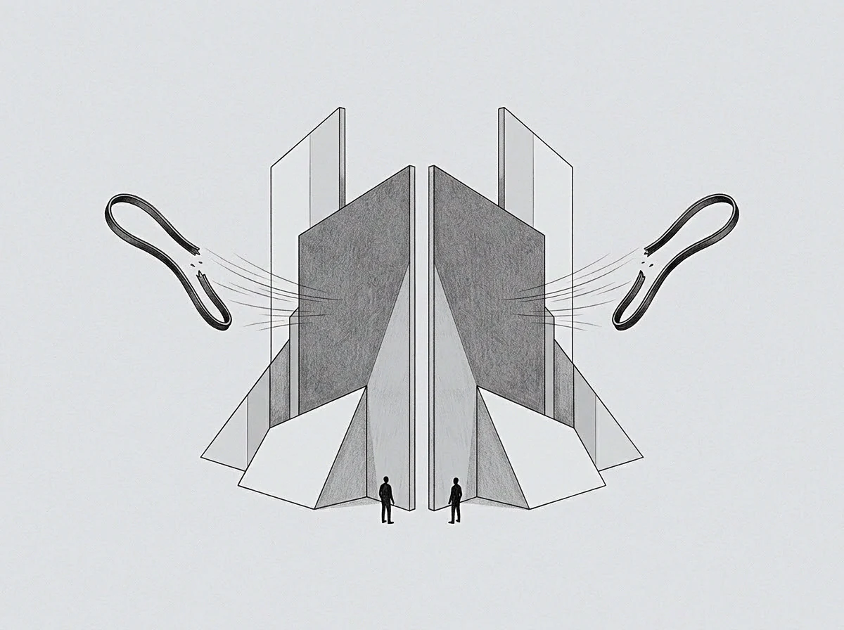
Clock
The dashboard showed thirty-two days of cumulative latency between strategic modification and downstream deployment. Strategic direction shifted in April, while technical execution continued along the prior trajectory until late May. The divergence created fifty thousand units of wasted throughput across three engineering teams.
Phase lag measures the temporal displacement between signal generation at an upstream origin and execution response at a downstream node. In coupled systems, this delay approaches zero. In decoupled execution topologies, the temporal displacement expands based on process cadence, validation cycles, and local buffering.
Every operational node maintains an internal execution clock. When two nodes operate without hard real-time synchronization, their internal clocks drift. The upstream node emits directives, specs, or capital allocations; the downstream node processes those inputs according to its local queue length and evaluation cycle.
Calculating the phase lag vector requires measuring both the temporal delay and the directional drift of execution output relative to the original signal.
The phase lag vector measures temporal displacement and directional divergence across asynchronous execution boundaries.
A static delay produces linear lag. Directional drift produces dynamic divergence where downstream work actively contradicts updated upstream targets. The cost of unmeasured phase lag expands as execution speed increases.
Rapid execution along an obsolete vector generates structural debt that demands costly remediation.

Temporal Coordinates and Local Cadence
Execution topologies decouple to maximize local autonomy and throughput. A software development unit operates on two-week sprint cycles. A corporate business development team operates on quarterly planning horizons.
A board of directors operates on annual budget allocations. These differing cycle lengths create baseline quantization delays.
Quantization delay defines the minimum waiting time before an upstream signal can enter a downstream execution queue. An update issued on day three of a ninety-day planning cycle sits idle for eighty-seven days before local evaluation begins. The minimum phase lag equals the remaining duration of the active downstream cycle.
Total lag accumulates as signals pass through successive decoupled layers.
Measuring phase lag begins with mapping local tick rates. The tick rate represents the frequency at which an execution node evaluates external signals and updates its internal backlog. Higher tick rates reduce temporal lag but increase evaluation overhead.
Lower tick rates reduce operational overhead while increasing temporal phase lag.
Failing to account for tick rate differentials causes severe organizational friction. Upstream teams assume instant propagation of strategic adjustments. Downstream teams process work according to local queue priority, unaware that upstream priorities shifted.
The resulting divergence costs capacity, capital, and execution momentum.

Skew
Phase lag vector computation relies on separating magnitude from direction. Magnitude represents temporal delay measured in hours, days, or operational cycles. Direction represents the angular discrepancy between the intended state vector and the realized execution vector.
Zero angular discrepancy indicates pure delay without structural misalignment. High angular discrepancy indicates that execution moved away from the target state.
Skew develops when local nodes reinterpret signals to fit existing baseline processes. A strategic directive to pause product expansion in favor of reliability work arrives at a feature team. The feature team continues building new components while refactoring internal APIs to satisfy the reliability directive.
The velocity vector contains ninety degrees of angular skew relative to the upstream intent.
Where Does Phase Lag Accumulate First?
Phase lag accumulates primarily at decoupled validation boundaries. When an execution unit completes a task, the output enters an evaluation buffer awaiting sign-off from an external authority. If the validation gate checks work against obsolete specs, phase lag doubles.
The downstream unit spends time completing work on an outdated trajectory, then spends equal time reversing that work after validation failure.
The following failure modes illustrate how phase lag vector components manifest across decoupled execution pipelines:
- Asynchronous Buffer Saturation occurs when downstream processing queues overflow, causing fresh upstream directives to drop or delay indefinitely while stale backlog items consume execution capacity.
- Spec Refinement Decay describes the loss of signal fidelity as directives pass through multiple managerial layers, increasing angular vector skew at each node.
- Validation Window Mismatch emerges when upstream evaluation cycles run on longer intervals than downstream iteration cycles, forcing downstream teams to build on unvalidated assumptions.
- Local Optimization Drift happens when local team performance metrics encourage continuous throughput along an obsolete path rather than idling to await updated instructions.
Quantifying these failure modes demands continuous monitoring of execution trajectories against upstream signal emissions. Linear tracking of task completion rates obscures phase lag. A team reporting one hundred percent velocity can simultaneously achieve zero alignment with current organizational priorities.
Angular skew converts pure temporal delay into active directional divergence across operational units.
The phase lag vector V is expressed as a function of delay duration t, signal decay rate d, and directional divergence angle theta. When theta exceeds ninety degrees, downstream execution actively undoes upstream value creation. The node spends operational energy climbing a negative value slope.
Downstream operators report completing tasks according to agreed metrics while upstream managers observe zero progress toward current targets.

Floor
Decoupled systems require a baseline variance floor to maintain execution stability. Attempting to force absolute zero phase lag across decoupled units destroys local autonomy. Real-time synchronization forces all nodes to run at the tick rate of the slowest layer.
The variance floor establishes the acceptable boundary of phase lag and angular skew before intervention triggers.
Calculating the variance floor involves assessing the cost of synchronization against the cost of drift divergence. In fast-moving environments, small phase lags carry low costs, making loose coupling optimal. In highly constrained regulatory or technical environments, small phase lags yield severe catastrophic outcomes, requiring tight synchronization bands.
The table below compares three primary execution topology configurations, their characteristic phase lag profile, and the associated operational metrics.
| Topology Configuration | Temporal Delay Range | Angular Skew Magnitude | Synchronization Cost | Unspent Capacity Potential |
|---|---|---|---|---|
| Synchronous Monolithic | Near Zero (Hours) | Minimal (0 to 5 degrees) | High Overhead | Low Latent Volume |
| Asynchronous Queued | Moderate (Days to Weeks) | Moderate (15 to 45 degrees) | Balanced Overhead | Moderate Latent Volume |
| Decoupled Autonomous | High (Weeks to Months) | Severe (45 to 120 degrees) | Low Overhead | High Latent Volume |
Establishing the floor prevents premature structural intervention. When phase lag stays within the floor boundary, local drift represents normal operational variation. When phase lag breaches the outer threshold, system architecture must force a alignment event.
System capacity remains trapped inside unaligned execution buffers until phase lag boundaries trigger synchronization events.
The boundary conditions defined in the execution contract establish when phase lag vectors require manual override.

Mesh
Modern organizations build complex execution meshes where nodes act simultaneously as upstream producers and downstream consumers. Signal routing in a mesh topology follows multiple paths. A single strategic shift propagates through technical, commercial, and operational vectors at different speeds.
The resulting phase lag distribution forms a multi-dimensional matrix.
Evaluating phase lag across a mesh requires analyzing every inter-node link. The longest path through the network defines the critical lag path. If product design lags engineering by two weeks, but legal approval lags marketing by twelve weeks, the legal-commercial link dominates the system phase lag vector.
Managing mesh lag relies on structured sequence protocols rather than arbitrary timeline compression. Execution flows through four distinct phases:
- Signal emission occurs at the origin node with explicit scalar and directional attributes.
- Queue ingestion takes place at the destination node during its regular tick evaluation cycle.
- Vector alignment checks the local queue against incoming signal vectors to discard obsolete tasks.
- Execution release commits local operational capacity to the updated state vector.
The path of least resistance across a mesh often leads nodes to skip stage three. Discarding work in progress feels expensive to local operators. Continuing obsolete work avoids the immediate discomfort of reporting lost throughput.
The local team protects its local performance metrics while compounding system-wide phase lag.
Avoidance acts as the primary coordinate marker for unprocessed phase lag. Where team interaction drops, phase lag accumulates silently. Unanswered technical queries, deferred API reviews, and unread spec updates mark the precise coordinates where execution vectors diverge.
The magnitude of avoidance reflects the volume of latent friction sitting behind the boundary.
Can decoupled nodes realign execution vectors without pausing active operational output?

Descent
Resolving phase lag vectors demands calculated directional realignment rather than abrupt halts. Halting execution flattens throughput and damages operational momentum. Effective realignment uses descent mechanics to guide local execution vectors toward the target trajectory along the path of least structural resistance.
A descent trajectory lowers angular skew incrementally across successive execution ticks. Rather than canceling all active downstream projects, the upstream node adjusts validation criteria for future tasks while allowing current work to drain through modified completion gates. The vector realigns smoothly without bursting queue capacity or causing operational panic.
Realignment succeeds when vector adjustment matches the natural drain rate of local execution queues.
The boundary of the current execution model defines what a system cannot process without structural failure. Pushing realignments beyond this boundary causes execution collapse, where teams lose trust in incoming directives and regress to ad-hoc local decision-making. Operating at the boundary edge yields maximum dynamic learning and model expansion.
Errors generated during vector realignment supply the exact coordinates required to refine system maps. Every failed handoff names a missing signal channel or an uncalibrated tick rate. Documenting these failure coordinates builds a precise map of organizational execution limits.
Measuring phase lag vector dynamics transforms organizational friction from a source of subjective frustration into a precise geometric input. Systems recover alignment when operators measure time and direction with identical rigor.
Optimal synchronization balances local queue velocity against structural directional alignment.