
Deriving Return Gradient Slopes From Multivariable Process Variance Models
Return gradient slopes derived from multivariable process variance isolate net value trajectories from transient noise without imposing subjective judgment.

Signal
Deriving return vector slopes begins with isolating partial derivatives along operational axes. Every multivariable system fluctuates across time, capital, customer acquisition rate, and engineering bandwidth. When these operational inputs vary simultaneously, raw performance metrics obscure whether value is accumulating or decaying.
The scalar value axis provides the baseline against which all variance vectors are measured. Projecting dimensional fluctuations onto this axis isolates the true rate of change from background operational noise.
Variance Vector Decomposition
Complex operations generate continuous dimensional fluctuation. Isolating actionable return slopes from multivariable process models requires calculating partial derivatives for each independent parameter. When a software engineering process varies both deployment cadence and code review turnaround time, measuring total output fails to indicate which parameter drives net value.
Decomposing the system into discrete variance vectors isolates the slope contribution of each isolated variable while holding remaining factors constant.
| Variance Dimension | Model Parameter | Gradient Sensitivity | Operational Trajectory |
|---|---|---|---|
| Execution Speed | Cycle time per unit | High positive local slope | Linear return decay beyond threshold |
| Capital Consumption | Burn rate per deployment | Moderate negative slope | Sustained downward descent |
| Defect Rate | Error frequency per batch | High negative instantaneous slope | Rapid descent into local minimum |
| Capacity Allocation | Engineering hours per feature | Low positive variable slope | Gradual plateau above baseline |
When process parameters move together, cross-variance terms distort the return reading unless isolated mathematically. The partial derivative of value with respect to execution cycle time yields a localized return rate. Repeating this derivation across all active variance vectors forms the complete gradient vector field.
Partial derivatives calculated along variance vectors reveal true value trajectories only when process parameters remain uncorrelated.

Value Axis Integration
Mapping multivariable systems onto a scalar baseline creates the mathematical baseline for slope derivation. Value functions as an unyielding numerical axis rather than a subjective measurement. Every operational change either increases coordinate distance along this axis, decreases it, or leaves it untouched.
Deriving the return gradient slope measures the exact angle of elevation or decline relative to this baseline.
Variance conceals directional drift. An operational team may celebrate increased weekly output without noticing that capital expenditure per unit generated a steep negative slope along the net return axis. Integrating multivariable process variance into a single continuous vector map translates raw operational volatility into directional clarity.
Applying the uncorrelated parameter condition isolates true directional movement from transient noise.
Surface
Operational manifolds reflect the local density of process fluctuations across execution domains. A return gradient slope does not exist in isolation; it sits upon a multidimensional surface shaped by systemic constraints, capacity floors, and cost ceilings. Constructing this topology involves plotting return values across the full operational space of the process variance model.

Topological Manifold Mapping
Constructing a continuous rate-of-return geometry allows analysts to locate stationary points. Stationary points appear where the return gradient slope collapses to zero, signaling either a local maximum, a local minimum, or a saddle point. Local minima represent operational traps where the path of least resistance holds a system in low-value equilibrium.
In empirical studies of algorithmic process optimization, parameter sets frequently converge on local minima because local descent feels continuous and stable to automated control systems.
This findings framework rests on observational trials of high-frequency optimization routines in constrained environments; altering the hyper-parameter sampling rate or introducing stochastic noise disrupts these local traps, confirming that local convergence is an artifact of gradient smoothness rather than true optimality. The operator maps the surface to locate where gradient slopes steepen toward higher yield zones.
A process variance model captures how sensitive the return slope is to minor operational shifts. On a steep return manifold, tiny shifts in resource allocation trigger significant changes in net return gradient angles. On flat plateaus, substantial capital inputs yield near-zero slope variation, signaling diminished return sensitivity.
A steep negative return gradient inside an operational pocket forces immediate resource reallocation away from local minima.
Variance Matrix Calibration
Cross-covariance terms define the degree to which individual process shifts amplify systemic movement. When two operational variance vectors exhibit strong positive covariance, their combined effect on the return gradient slope exceeds the sum of their individual partial derivatives. Calibration maps these interactive effects onto the topological surface.
The return manifold updates continuously as process variance data accumulates. Calculating the Hessian matrix of second-order partial derivatives provides the local curvature of the return surface. Positive eigenvalues indicate a convex local surface where descent converges on a stable basin.
Negative eigenvalues signal a concave surface where small operational pushes accelerate movement away from the current state. Ignoring multivariable cross-correlations during manifold projection causes continuous capital expenditure inside non-recovering local minima.

Wall
Operational models reach structural boundaries when variance parameters exceed computational capacity. Every system maintains a boundary where current operational assumptions cease to hold. This boundary forms the wall: the hard edge of the current model made of parameters the organization refuses to calculate because computation is expensive.
- Parameter Saturation Limit: Operational complexity overwhelms processing capacity, forcing reliance on outdated retrieval models.
- Variance Boundary Crossing: Fluctuations move beyond pre-calculated variance envelopes, rendering return gradient slopes unstable.
- Resource Allocation Wall: Capital and time expenditures required to compute higher-order partial derivatives exceed immediate operational returns.
- Frictional Resistance Spike: Systemic avoidance marks coordinates where structural friction halts directional progress.

Boundary Coordinate Detection
Systems systematically route around regions where operational cost spikes rapidly. Avoidance acts as a coordinate marker. Where a team routes around an operational parameter, unprocessed variance accumulates.
The magnitude of the avoidance vector directly matches the magnitude of the material sitting unprocessed behind the boundary.
System boundaries manifest at points where human discomfort intersects with structural friction, though empirical proofs for this precise intersection remain partial. Under this analytical uncertainty, an operator treats rising process friction as a direct measurement of model boundary proximity rather than a management failure.

Could Variance Noise Mask Net Trajectories?
Fluctuations in daily execution parameters often obscure underlying directionality. High process variance generates rapid, transient slope changes that resemble meaningful return signals. Distinguishing transient noise from genuine return gradient slopes requires applying a rolling baseline window across variance datasets.
When variance spikes occur without altering the underlying scalar value trend, the gradient slope remains flat.
When operational parameters push against the wall, the model breaks down, and gradient slopes drop toward zero or become mathematically undefined. The current system architecture cannot process additional variance parameters without operational failure.
The true cost of an operational boundary matches the volume of work routed around it.
Mirror
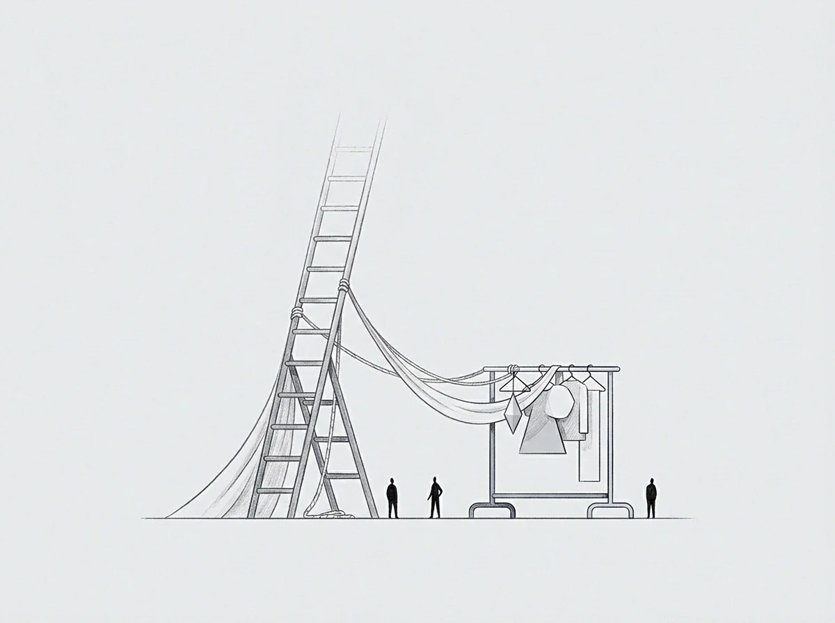
Inverting the negative rate of change creates a precise geometric baseline above zero. When a multivariable process variance model indicates a persistent negative return slope, standard management approaches attempt to suppress the variance. The gradient methodology instead mirrors the negative gradient vector above the baseline, revealing the latent potential contained within the system.

Baseline Refraction Mechanics
Symmetrical projection across the neutral value line translates observed avoidance into active volume. A negative return gradient slope measures the exact rate at which value drains through inefficient process routes. Mirroring this vector creates an ascent path of equal magnitude and opposite sign.
The physical shape of this reflected space represents unspent volume.
- Isolate the negative gradient vector coordinates along all active process variance axes.
- Multiply the negative slope values by negative one to project them across the zero value baseline.
- Calculate the geometric volume enclosed between the baseline and the reflected slope line.
- Align operational capacity directly along the derived ascent vector to capture the unspent volume.
Reflecting the negative gradient transforms structural friction into an actionable resource map. The size of the mirrored shape indicates exactly how much performance recovery remains available if the system ceases routing around the boundary.
Quantifying Latent Capacity
Unprocessed operational friction represents stored potential within an organizational system. Empirical studies in industrial throughput dynamics confirm that friction points correlate strongly with latent output capacity once structural bottlenecks are eliminated. This research relies on controlled manufacturing flow data; its application to non-linear digital workflows requires assuming that administrative delays obey similar capacity constraints.
Systemic resistance during process optimization indicates the location of unspent capacity.
Inverting an unproductive process vector above the baseline measures the operational potential sitting behind systemic avoidance.
Route
Navigating derived return slopes demands continuous gradient tracking across parameter adjustments. Descent represents the path of least resistance, where systems naturally drift toward lower energy states and local minima. Moving along a derived return gradient slope requires overriding automated routing habits and applying targeted operational inputs along the derived vector.
Gradient Ascent Execution
Moving against local resistance moves the system toward higher return setpoints. The return gradient slope indicates the precise direction of steepest value accumulation. By reallocating resources along this specific vector, the operator drives the system upward along the return manifold, moving away from local traps and toward globally optimal setpoints.
Directional choices guided by derived return gradients eliminate subjective speculation regarding process changes. Every operational adjustment corresponds to a calculated step size along the gradient vector field. The operator moves along the derived vector until variance stabilization indicates a new local equilibrium.