
Estimating Heavy Tail Exponents From Unordered Asset Drawdowns
Stripping chronological order from peak-to-trough drawdowns isolates tail thickness through rank-frequency decay while shifting serial clustering into parameter bias.

Descent
A terminal screen lists sixty-two peak-to-trough losses across ten years of trading, stripped of their calendar stamps and sorted by nothing at all. The operator looking at the figures sees no dates, no bull markets, and no monetary policy cycles, only a raw heap of downward excursions from previous equity peaks. Standard risk accounting ties drawdowns to dates and seasons on a timeline.
When an operator strips out that chronological dimension, the data becomes an unranked sample of negative excursions where each point is simply a fractional decline from an earlier high-water mark to a trough.
Losses accumulate downward along the value axis. In mathematical optimisation, every trading strategy searches a noisy surface: building value requires execution, discipline, and energy, while the downward slide follows the path of least resistance. When capital pulls out of an asset, it follows liquidity downhill.
Removing chronological sequence isolates that downward pull, giving an operator an unvarnished view of the model’s tail behavior without the comforting fiction that time alone restores an equity curve.

Drawdown Magnitudes On The Value Axis
Peak equity establishes the benchmark from which every subsequent drop is measured. A drawdown begins the moment an asset dips beneath its historical peak and closes only when price clears a new high. In liquid markets, the depth of these drops does not follow a Gaussian distribution; large dislocations happen far more regularly than bell curves allow.
The tail decays as a power law, meaning the odds of an excursion larger than x scale proportionally to x raised to a negative exponent alpha.
Unordered drawdown sets strip chronological relief and leave raw terminal losses exposed on the value axis.
The parameter alpha serves as the heavy tail exponent. A large alpha means probability decays quickly and catastrophic drops remain outliers. A small alpha concentrates probability mass in extreme events, showing that deep drawdowns are structural properties of the strategy rather than transient shocks.
Estimating alpha accurately gives an operator the real probability of ruin. By stripping consecutive losses of their sequence, the analyst can treat historical drawdowns as independent draws from an underlying tail distribution to evaluate structural vulnerability directly.

Stripping Time From The Negative Slope
Treating drawdowns as an unranked set strips away the psychological cushion of recovery periods, where rallies visually offset prior crashes on a chart. Without a calendar axis, fifty percent drops sit directly alongside three percent pullbacks, turning a conventional timeline into a pure density profile. This arrangement clarifies whether the asset exhibits Pareto-type tails, separating strategies that merely leak operational friction from those vulnerable to complete collapse.
Unordered drawdowns behave quite differently from daily return series. Daily returns capture single-period differences, whereas drawdowns track cumulative, path-dependent declines that resolve only when the asset sets a fresh high. Because a drawdown compounds several negative return periods, its distribution typically carries a heavier tail than the underlying returns.
Evaluating them without sequence forces an analyst to treat the cumulative slide as a single physical realization of downside exposure, where the contractual terms governing high-water resets determine whether consecutive drops register as separate events or legs of a single protracted collapse.

Threshold
Setting the cutoff k in an empirical distribution balances sample variance against systematic bias. Extreme value theory shows that power-law behavior emerges only above a certain depth. Set the threshold too low, and the sample gathers routine pullbacks from the Gaussian center, drowning the calculation in ordinary noise.
Push it too high, and the sample dwindles to two or three points, sending the estimator’s variance out of control.
Engineers do not size suspension cables using the average weight of commuter traffic; they design for load spikes from gale-force winds and freight lines, ignoring routine oscillations. Portfolio drawdowns require the same filter. A standard five percent dip reveals nothing about how a fund survives a liquidity freeze.
The calculation has to isolate the genuine tail, locating the empirical boundary where power-law decay takes over.

Extreme Value Cutoffs And The Hill Plot
Bruce Hill’s log-log ratio calculates the tail index directly from upper order statistics. After sorting the unordered drawdowns from smallest to largest, the analyst isolates the k largest observations. The Hill estimator takes the average logarithmic difference between each extreme observation and the chosen cutoff, and plotting this across values of k produces the Hill plot.
The goal is to locate a stable horizontal plateau where the estimated exponent holds steady as the cutoff shifts.
Setting the upper order statistic cutoff too deep into the body of the distribution introduces systematic sample bias into the estimated Pareto exponent.
The Hill estimator’s asymptotic normality rests on independent, identically distributed Pareto-type observations and intermediate sequence conditions on the upper order statistics. Empirical dependence across asset drawdowns from clustered volatility breaks this consistency, requiring block bootstrap testing across high-frequency equity ticks to falsify. When serial correlation persists in the underlying returns, drawdowns become dependent excursions that skew the Hill plot up or down, dissolving the plateau into an unstable curve that resists visual interpretation.

Where Does Calibration Fail In Extreme Excursions?
Serial dependence between consecutive declines compresses the effective degrees of freedom in heavy-tailed data. When an asset suffers a deep structural break, the initial recovery frequently stalls, generating overlapping troughs that risk models routinely mistake for independent observations. Compiling unordered drawdowns without declustering creates three distinct calibration breakdowns:
- Pseudo Independent Clustering occurs when secondary drawdowns occurring within an unresolved broader bear market are recorded as distinct events, artificially inflating the sample size with correlated observations.
- Threshold Contamination arises when the analyst includes routine operational churn below the true Pareto transition point, producing an overestimated alpha that understates systemic tail thickness.
- Finite Sample Truncation restricts the upper tail observation count, causing heavy-tailed models to underestimate the probability of losses larger than the historical sample maximum.
Risk professionals frequently divide over whether to automate threshold selection or rely on visual inspection of mean excess plots. Algorithms optimize formal goodness-of-fit criteria but tend to latch onto local numerical artifacts. Manual review incorporates context about past market regimes, yet it introduces operator bias.
The unresolved problem is whether automated routines can identify the true Pareto transition point without manual assessment of shifting volatility regimes.

Table
Empirical evaluation of tail estimators reveals clear trade-offs across unordered loss samples. Each mathematical framework negotiates bias, variance, and sample size through a different structure. To guide how an operator selects a tool for unordered drawdowns, four primary approaches are compared below across their operational constraints and sensitivities.
| Estimator | Structural Assumption | Bias Vulnerability | Sample Size Demands |
|---|---|---|---|
| Hill Estimator | Exact Pareto tail behavior in upper order statistics | High sensitivity to choice of threshold k | Moderate sample size exceeding fifty tail observations |
| Pickands Estimator | Generalized extreme value domain of attraction | High variance in intermediate sample fractions | Large sample size exceeding two hundred observations |
| Maximum Likelihood GPD | Peaks over threshold follow Generalized Pareto Distribution | Moderate bias under misspecified tail cutoffs | Moderate sample size with stable numerical convergence |
| Gabaix-Ibragimov Regression | Log rank log size linear scaling with rank shift | Low sensitivity to small sample downward bias | Small sample size viable down to thirty observations |

Estimator Performance In Unordered Samples
Each formulation reacts differently when pooled drawdowns contain latent volatility clustering. The Hill estimator remains standard due to computational simplicity, yet its threshold sensitivity introduces meaningful operational vulnerability. The Pickands estimator avoids strict Pareto assumptions by operating across the broader extreme value domain.
The Pickands estimator’s consistency rests on extreme value index bounds between negative one-half and positive one-half, tested on stationary financial returns. Heavy-tailed drawdowns with exponents below unity invalidate the moment convergence, an outcome proven false if finite higher-order moments emerge in prolonged secular bull regimes.
Maximum likelihood applied to the Generalized Pareto Distribution solves for scale and shape simultaneously. This paired parameterization accommodates distributions that shift gradually from exponential decay into fat power-law tails by optimizing the likelihood function across every point past a threshold u. While flexible, numerical solvers often fail to converge when working with sparse samples or outsized outliers that warp the likelihood gradient.

Rank Frequency Regressions In Small Samples
Regressing log rank on log size provides a direct estimate of the tail exponent, but ordinary least squares introduces negative bias into the standard errors. Standard Zipf regressions arrange unordered drawdowns in descending order, giving rank one to the worst drop. In small samples, however, standard log-log fits systematically overstate tail thickness because correlated error terms among higher-ranked observations violate classical regression assumptions.
Xavier Gabaix and Rustam Ibragimov addressed this distortion by substituting the integer rank r with the quantity r minus one-half. That simple offset neutralizes the leading-order bias of the ordinary least squares slope. When working with seventy unordered drawdown observations from a private fund track record, this adjusted regression provides a robust, practical alternative to numerical maximum likelihood.
The one-half rank shift stabilizes the fit across fragmented trading histories without overfitting the tail.

Mirror
Inverting the tail exponent across the baseline shows the volume of unhedged capital exposed to ruin. In physical systems, potential energy equals the work needed to lift a mass against gravity; in financial risk, reflecting a negative tail exponent above the baseline outlines the latent loss exposure inside the portfolio. An operator tracking only realized gains misses this mechanism.
The downward gradient marks the channel through which capital drains during stress, and mirroring that curve yields a quantitative boundary for latent tail risk.
Thin tails decay exponentially, keeping extreme losses improbable enough that a desk can operate on lean cash buffers. Power-law tails decay far more slowly. While pooling drawdowns across disparate assets can help preserve an underlying Pareto profile, shifts in market regimes alter systemic tail thickness; under that uncertainty, the risk officer fits separate exponents across isolated liquidity regimes and assigns capital reserves to the thickest observed tail.
When drawdown excursions follow power law distributions, scaling the tail index below two eliminates the mathematical expectation of portfolio variance.

Latent Potential And Power Law Decays
Heavy-tailed profiles signal that severe downside momentum remains stored behind routine market swings. Where an operating strategy redirects its attention indicates where unhedged exposure gathers. A fund that routinely caps daily fluctuations often accumulates severe latent risk to discontinuous market breaks: minor pullbacks are trimmed and managed through active trading, while structural drops remain unhedged because protective carry depresses daily returns.
This dynamic builds unmonitored loss capacity beneath the surface, a volume measured directly by alpha. As alpha nears unity, the expected value of a drawdown expands toward the entire fund valuation. An alpha below unity describes an environment with an unbounded theoretical mean loss, where a single drawdown will eventually consume the full asset base over time.
Calculating alpha from unordered drawdowns marks the exact boundary where the prevailing risk model breaks down.

The Boundary Of The Finite Variance Regime
When the estimated alpha drops below two, classical portfolio theory based on mean and variance stops working. The central limit theorem requires finite variance for sample averages to converge on population parameters; below two, variance expands without an upper limit. Under those conditions, metrics like the Sharpe ratio, standard deviation, and standard value-at-risk calculations mask catastrophic exposures.
The framework distinguishes four operational states defined by the tail exponent:
- Exponential Regime where alpha diverges toward infinity, confining drawdowns to narrow Gaussian boundaries that permit conventional leverage.
- Finite Variance Pareto Regime where alpha sits between two and four, allowing variance metrics to stabilize while kurtosis remains heavy and volatile.
- Infinite Variance Regime where alpha falls between one and two, destroying the mathematical validity of mean-variance portfolio optimisation and necessitating physical cash buffers.
- Infinite Mean Regime where alpha drops below one, indicating that the theoretical expectation of loss is infinite and making solvency mathematically impossible under long-term exposure.
Every tail estimate carries operational friction. When historical drawdowns indicate an alpha of one point four, standard hedging formulas fail. Portfolio rebalancing routines driven by covariance matrices direct capital into assets whose downside exposure is mathematically unbounded.
Bypassing liquidation metrics avoids pricing discontinuous price gaps, turning any portfolio with a tail index below the finite variance threshold into an unhedged bet on bottomless liquidity.

Cost
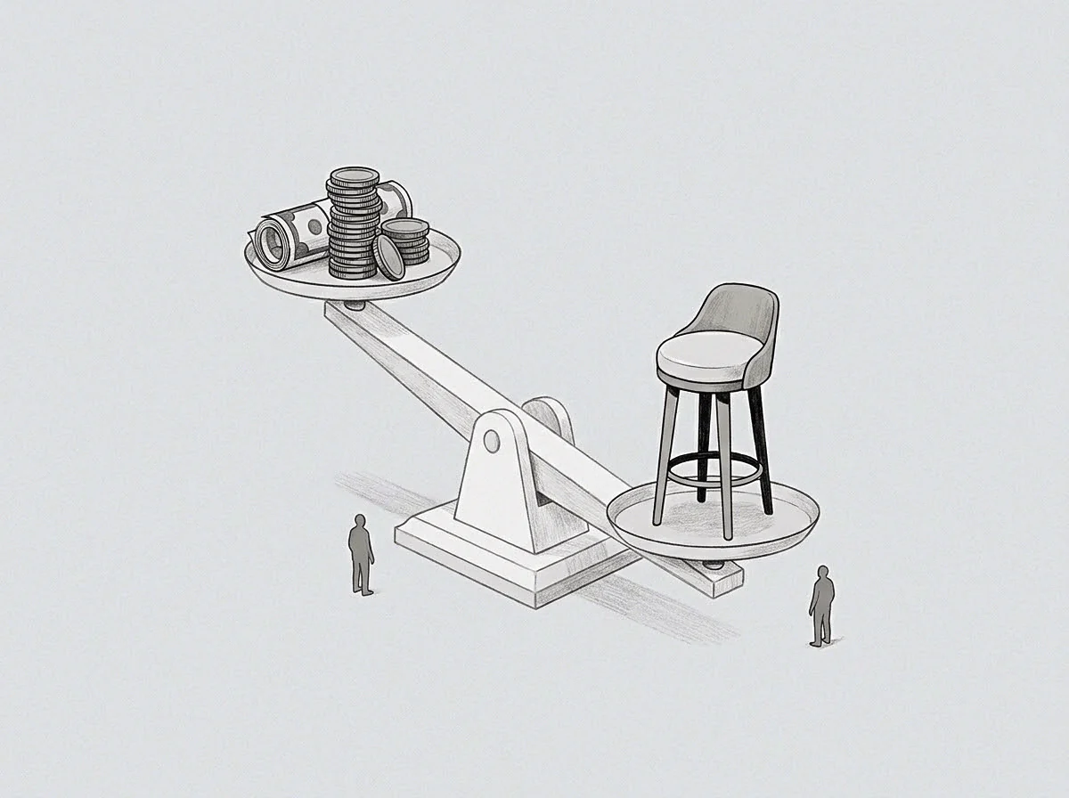
Underestimating tail thickness drains risk capacity long before formal liquidation begins. When a fund sizes its leverage against a thin-tailed model, a single severe dislocation quickly breaches maintenance margin limits. The tangible cost appears as depleted collateral, drained liquidity, and surrendered operating autonomy as the clearinghouse liquidates the account.
Miscalculating alpha demonstrates that the tail exponent is not an academic exercise; it marks the boundary between continued trading and institutional failure.
As asset declines accelerate, liquidity drains from secondary books, steepening the loss curve. A model calibrated exclusively on tranquil periods hits a wall when live execution diverges from paper assumptions. When prices gap downward past stop-loss thresholds, portfolio insurance breaks down because no buyers stand ready to take the other side of the trade at the modeled marks.
Capital Depletion Under Heavy Tails
Severe drops rarely develop in orderly steps; they arrive in discontinuous breaks that exhaust liquidity reserves. When relying on unordered drawdowns to evaluate strategy survival, the resulting tail exponent governs the required cash allocation. A fund trading heavy-tailed assets cannot rely entirely on dynamic hedging.
Unallocated cash must sit in short-term government paper, serving as an inert shock absorber against outsized market moves.
Thick tail exponents require capital reserves determined by maximum historical excursions rather than smoothed moving averages.
Carrying large cash reserves incurs an ongoing performance drag, lowering gross returns throughout sustained bull markets. Operators encounter steady pressure from allocators to deploy that idle liquidity to enhance short-term yield at the expense of survivability. Resisting that pressure rests on the mathematics of heavy tails, where the estimated alpha shows that a severe drawdown becomes an inevitability across a long enough operating horizon.

The Wall Of Liquidation Limits
Every fund operates against a ceiling imposed by prime broker agreements and clearinghouse mandates. That threshold represents the hard boundary of the business model, where an overshoot triggers forced liquidation. Sizing the heavy tail exponent from unordered drawdowns tracks the true buffer between present capital and that liquidation floor.
When the exponent enters the infinite variance zone, internal discipline alone cannot prevent margin depletion unless the desk cuts gross exposure.
The entire financial burden of misreading tail thickness falls on the equity holders. Prime brokers protect their positions by liquidating collateral the moment maintenance marks fail, locking in losses at the trough of the cycle. An operator who underestimates alpha surrenders the seat, the firm, and years of accumulated gains over a few volatile sessions.