
Evaluating Operational Variance Using Baseline Return Gradient Analysis
Baseline return gradient analysis evaluates operational variance by calculating the directional rate of output change relative to an empirical baseline plane.
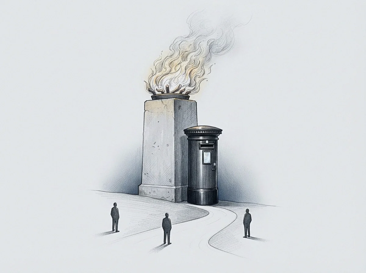
Signal
An operations log recorded seventy consecutive days of throughput decline while gross margins remained fixed. Operating staff tracked output volume alone, treating steady invoice totals as proof that performance remained unchanged. Beneath the balance numbers, input resource consumption per completed unit rose fourteen percent over the period.
A system operating under static return metrics conceals directional drift when inputs shift faster than output realizations.
Baseline return gradient analysis measures the local derivative of realized return against the vector of operational variance. Operational changes produce directional displacement across capacity, labor allocation, capital expenditure, and processing cycles. The baseline represents an empirical plane of nominal operating efficiency established under controlled conditions.
Evaluating variance through gradients calculates the slope of efficiency loss or gain per incremental step away from this reference plane. That slope shows whether an operation moves along a path of least resistance or burns excess capacity to sustain the illusion of a level trajectory.
A gradient measurement maps the directional rate of output change per unit of operational displacement from a verified baseline.
Traditional variance analysis calculates cardinal differences between planned budgets and actual ledger totals. Ledger reconciliation arrives after cycles conclude, registering financial aftermath without recording the slope of operational decay. Return gradient analysis operates continuously across the ordinal execution state, showing immediately whether an operational adjustment adds friction regardless of lagging revenue reports.
Treating gross return as an isolated metric obscures the internal incline of operational erosion until recovery demands total process reconstitution.

Post
Structural reference points anchor gradient evaluation. A fixed post defines the baseline parameters: unit labor duration, material input velocity, queue latency, and error remediation intervals. Deviations occur along these axes simultaneously.
Measuring variance requires comparing the aggregate vector of these displacements against the baseline plane rather than examining isolated line items.
When an operating team changes routing procedures to bypass an internal bottleneck, local process speed improves, but upstream buffer accumulation increases simultaneously. The local calculation registers progress; the baseline return gradient registers aggregate descent. The system routes around the friction point, accumulating unprocessed work elsewhere in the workflow.
| Variance Dimension | Observed Vector | Baseline Return Gradient | Structural Consequence |
|---|---|---|---|
| Queue Latency Expansion | Positive displacement in buffer dwell time | Negative slope relative to capital utilization | Working capital locks into inactive inventory states |
| Labor Intensity Substitution | Higher touch time per finished unit | Steep downward gradient against capacity margins | Capacity ceilings drop across adjacent production lines |
| Routing Bypass Protocol | Shortened primary path cycle | Negative aggregate return across error remediation | Unprocessed latent defects emerge in downstream assembly |
| Parameter Drift Acceptance | Relaxation of entry tolerance thresholds | Flat initial gradient transitioning to sharp drop | Terminal inspection reject rates climb exponentially |
The coordinate position of an operation along its performance curve depends on structural limits. A process parameter set outside specified tolerance bands invalidates baseline assumptions and forces an immediate recalibration of the baseline gradient equation.
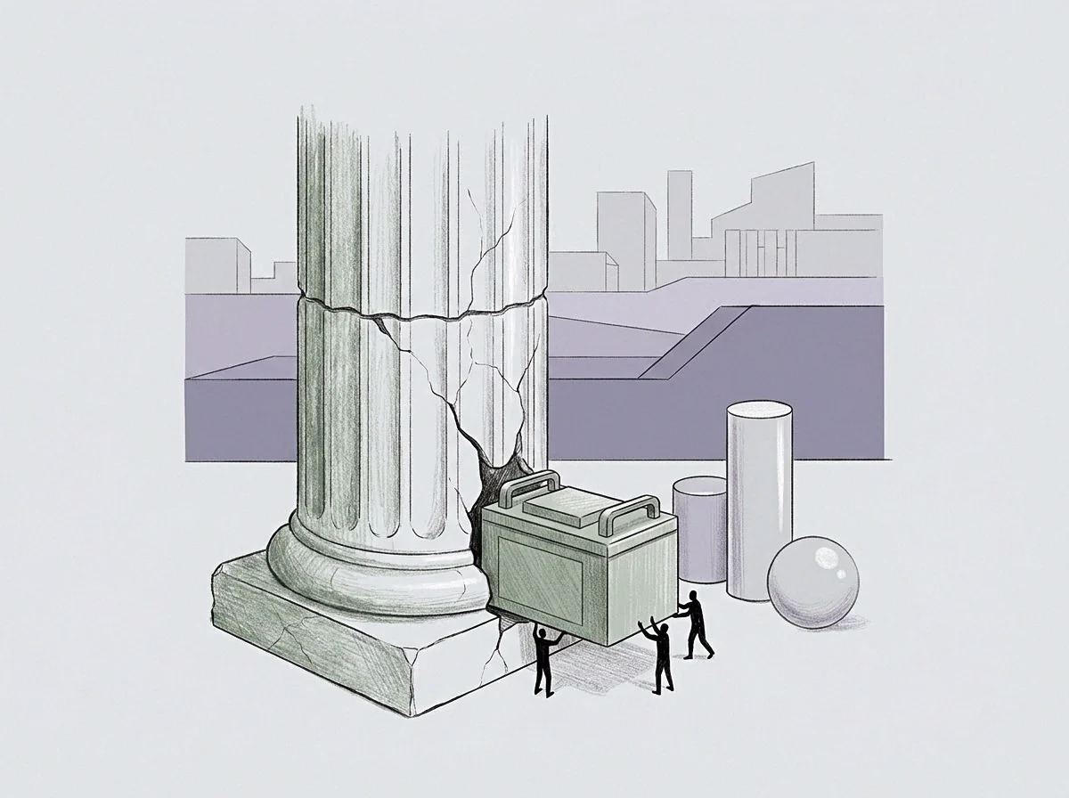
Incline

Is Baseline Rate Divergence Measurable Without Cardinal Loss?
Rate divergence registers in system geometry before financial loss appears. Take an enterprise software deployment facility with ten implementation engineers as a worked situation. The baseline plan assumes forty hours of deployment labor per client instance, yielding an expected return rate of five operating units per week.
Over twelve weeks, total completed deliveries remain stable at five units weekly. Client satisfaction ratings remain unchanged, and invoice figures match budget expectations exactly.
The operational vector reveals divergence. Engineering hours spent per deployment rise from forty to fifty-eight. The team compensates for configuration friction by absorbing unlogged weekend hours and rerouting senior architect time into routine script execution.
The baseline return gradient reveals a steep negative slope: return per labor hour drops thirty-one percent despite steady cardinal output. This incline measures the consumption of reserve capacity.
Operational stability during input inflation marks an uncredited expenditure of reserve capacity.
Evaluating this variance identifies four structural components within the gradient calculation:
- Displacement Magnitude tracks the absolute distance between baseline operating coordinates and current parameter allocations across time.
- Directional Vector identifies which specific operational factors consume excess capacity to maintain output targets.
- Return Incline calculates the differential rate of yield per unit of added operational friction across the workflow.
- Latent Deficit quantifies the volume of deferred maintenance and human exhaustion accumulating behind temporary workarounds.
Ascent requires deliberate operational investment. Left unmanaged, systems descend along the path of least operational resistance.
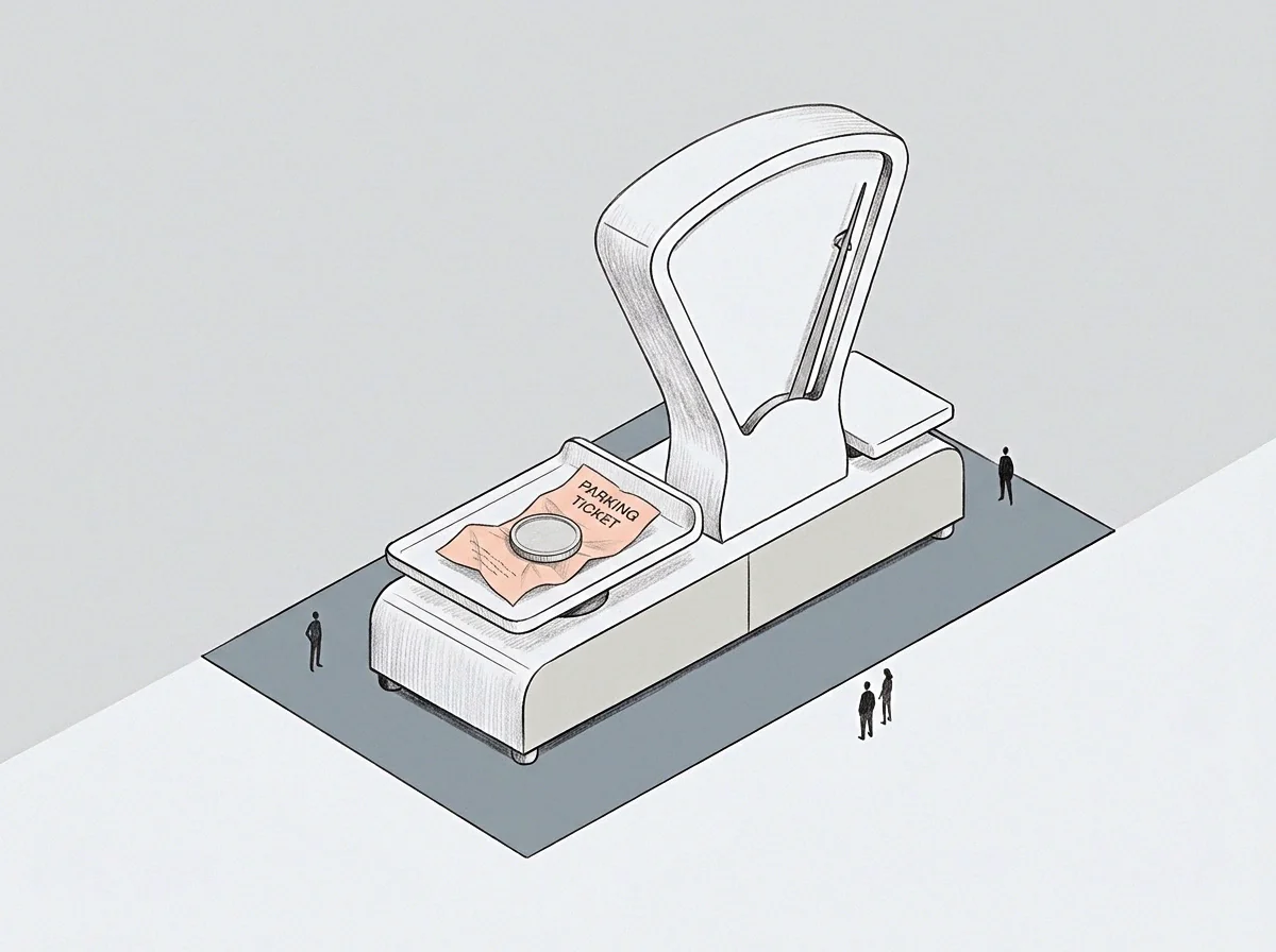
Boundary
Every operating model functions within structural boundaries. The boundary represents the limit where current operational logic stops yielding solutions and begins generating compounding errors. Systems resist pressing against this wall because operational redesign demands substantial capital, attention, and systemic reorganization.
In cold-rolling metal mills, roller bearings endure mechanical stress within verified pressure envelopes. Operators monitor thermal gradients across bearing housings. When friction elevates temperatures toward metal phase-transformation points, operators slow the strip speed.
The reduction preserves the tool while reducing hourly volume. Industrial machines register physical boundaries through thermal elevation and vibrational harmonics.
A process boundary marks the exact coordinate where current operating architecture fails to absorb variance without structural degradation.
Human operating systems exhibit identical dynamics. When an administrative workflow encounters a boundary, operators introduce manual checks, side spreadsheets, and informal communication channels. These informal adaptations function as heat dissipation mechanisms.
They route around the boundary while the underlying model remains rigid.
The operational baseline will accommodate these adjustments for another quarter without structural intervention.

Tally
Evaluating operational variance converts gradient readings into concrete structural adjustments. The process separates temporary environmental disturbances from systematic baseline shifts. Temporary disturbances cause localized variance spikes that decay back toward baseline coordinates without procedural intervention, whereas systematic shifts alter the underlying return gradient permanently.
Calibration follows an orderly sequence of operational corrections:
- Parameter Logging establishes real-time recording of input vectors alongside gross output figures to identify early coordinate drift.
- Gradient Derivation calculates the mathematical slope of return per unit change across all monitored operational variables simultaneously.
- Boundary Mapping locates the exact process constraints causing negative return gradients through structured capacity testing.
- Setline Reconstitution resets baseline operating parameters to match current structural realities rather than historical assumptions.
The data demonstrates clear slope deterioration. How much latent potential remains recoverable once an operational descent is fully mapped across the organization?