
Measuring Marginal Return Rates On Incremental Enterprise Capital
Marginal return rate measures net change in enterprise return gradient generated by the final unit of deployed incremental capital.

Baseline
Evaluating marginal return rates on incremental enterprise capital demands pulling apart two operational dynamics frequently treated as identical: the immediate revenue output generated by adding funds to an existing line, and the structural shift in the enterprise return gradient caused by that expenditure. Enterprise capital allocations often show high nominal yields in early reporting periods. This initial gain occurs because primary injections harvest pre-existing operational capacity.
Accounting yields measure gross output against capital input, failing to isolate whether deployment expanded the underlying system or merely accelerated the consumption of latent efficiency.
Establishing an accurate baseline return rate demands measuring enterprise performance across static operational windows before introducing secondary capital infusions. When an enterprise deploys capital into a functional unit, the immediate rate of return reflects both the inherent productivity of the asset and the structural friction of the surrounding enterprise architecture. Measuring incremental capital performance without subtracting baseline friction produces inflated expectations.
The true marginal return rate represents the precise derivative of the yield function with respect to the incremental capital unit deployed.
A baseline return rate reflects historical capacity before incremental capital shifts the enterprise friction profile.
Revenue growth masking margin decay creates misallocation. When capital enters an enterprise system, internal coordination costs rise non-linearly. A sales team expanded by fifty percent may generate thirty percent more top-line revenue, but the internal administrative load created by that expansion reduces net operational margins across adjacent departments.
Measuring the marginal return on that capital injection solely through the sales team balance sheet obscures enterprise-wide erosion. The baseline calculation must account for systemic absorption capacity prior to capital entry.
A six-month baseline observation window isolates baseline variance from incremental capital effects.

Seat
The operator sitting in the capital allocation seat faces a persistent structural distortion: short-term financial metrics reward direct deployment into revenue-producing assets, while systemic capacity limits dictate long-term return rates. Accounting profit reflects prior operational choices. Consider a capital allocation decision within a mature logistics business operating with ten million dollars in annual capital expenditure.
Assume the enterprise allocates two million dollars in incremental capital across two distinct paths over a twenty-four month evaluation period:
- Capacity Expansion Allocation: Funds injected directly into existing fleet assets yield immediate top-line expansion while internal dispatch coordination costs compound quietly.
- Structural Efficiency Allocation: Capital committed to internal automation lowers baseline unit costs, raising the long-term enterprise capital absorption slope.
- Buffer Preservation Allocation: Capital retained in reserve prevents forced debt issuance during operational friction spikes.
In the first path, the two million dollars purchases additional transport vehicles. Top-line revenue rises by twelve percent within ninety days. Dispatch systems, vehicle maintenance bays, and administrative teams experience severe operational pressure.
The unit cost per delivery increases by seven percent across the entire fleet. The marginal return rate on the incremental two million dollars appears positive on a direct departmental yield basis, yet enterprise net margin drops by ninety basis points as static yields obscure systemic friction and capital absorption drops with expanding complexity.
Unstated operational capacity constraints transform linear capital injections into diminishing return curves.
In the second path, the operator directs the two million dollars toward software automation and maintenance facility workflow restructuring. Direct revenue generation during the first two quarters remains flat. Enterprise unit delivery costs drop by four percent in quarter three, increasing net operating income across the pre-existing ten-million-dollar asset base.
The incremental capital generates a marginal return rate far exceeding the enterprise cost of capital by altering the operational slope rather than adding volume to a clogged process.
The additional capital was supposed to double capacity rather than consume administrative hours.

Slope
Computing the enterprise return gradient requires mapping the incremental rate of return against total capital volume deployed. When incremental injections yield progressively smaller output gains, the system enters a regime of diminishing returns. Capacity boundaries constrain capital velocity.
Mapping this slope allows capital allocators to identify the exact threshold where secondary expenditures destabilize existing enterprise margins.

Mapping Capital Absorption Mechanics
Capital deployed into an enterprise interacts with structural constraints. Operational limits dictate terminal return rates. Friction accumulates at handoff points between operational units, software layers, and governance structures.
An initial capital injection encounters low friction, producing high direct return rates. Secondary and tertiary injections face compounding internal resistance. The slope of the return curve turns negative long before gross enterprise revenue begins to decline.

Evaluating Comparative Allocation Paths
Evaluating marginal return rates across contrasting deployment modes requires tracking systemic variables alongside direct financial yield. The table below details structural parameters across direct expansion capital and structural efficiency capital within a standardized enterprise environment.
| Deployment Attribute | Direct Scaling Capital | Efficiency Structuring Capital |
|---|---|---|
| Initial Cash Yield Acceleration | Immediate high top-line realization | Delayed baseline margin realization |
| Enterprise Coordination Overhead | Compounds non-linearly with volume | Decreases per unit of output |
| Capital Absorption Ceiling | Constrained by operational bottlenecks | Expands total enterprise capacity limit |
| Measurement Lag Window | Short thirty to sixty day feedback cycle | Extended six to twelve month observation window |
| Terminal Return Rate Profile | Sharp decay at capacity boundary | Asymptotic stabilization above baseline |
Systemic constraints govern marginal yield limits. Direct scaling capital delivers quick feedback metrics, tempting decision-makers to commit excess capital into declining operational gradients. Efficiency capital exhibits long measurement lags, masking early capacity improvements behind flat short-term revenue performance.
Measuring marginal return rates demands tracking operational friction velocity alongside direct cash output.
Unspent volume mirrors historical resistance. When enterprise capital allocations bypass structural bottlenecks, accumulated friction redirects into downstream administrative processes, compounding enterprise coordination expenses.
Miscalculating the return gradient results in stranded capital liabilities across overburdened operational units.

Lag
Measurement lag distorts incremental return calculations. Financial reporting operates on fixed monthly or quarterly cadences, whereas operational friction manifests across multi-quarter cycles. Capital injected into enterprise expansion shows deceptively high early efficiency because organizational systems absorb short-term stress before operational failure occurs.
Unprocessed friction accumulates along operational paths.

When Does Incremental Capital Produce Negative Gradient Shift?
A negative gradient shift occurs when the enterprise coordination cost generated by a new capital asset exceeds the net operating income produced by that asset. Incremental allocations exhaust easy efficiency gains. Consider an enterprise expanding its regional fulfillment centers.
The fourth center increases network capacity by fifteen percent, but raises multi-facility inventory balancing costs across the entire logistics footprint by twenty-two percent. The marginal return rate on that fourth facility is negative on an enterprise basis, despite the individual center posting positive local operating earnings.

Accounting Distortions in Extended Windows
Standard enterprise balance sheets fail to capture the temporal decay of capital efficiency. The sequence of operational decay follows a predictable progression:
- The initial injection yields immediate revenue output without immediate overhead expansion.
- Operational complexity accumulates across administrative and technical systems over subsequent cycles.
- Marginal yield drops below internal hurdle rate as coordination friction consumes incremental capacity.
Structural decay alters baseline projections. Delaying capital measurement until annual reporting cycles allows misallocated expenditure to compound across multiple operational quarters. Return velocity slows near structural walls.
Effective capital evaluation demands continuous monitoring of unit operating margins throughout the capital deployment lifecycle.
Capital injected into a saturated channel produces nominal growth while depressing the overall enterprise return gradient.
Tracking return velocity over time exposes structural friction before financial statements record yield decay.

Scale
Enterprise capacity boundaries form rigid structural limits. When capital expenditure approaches the boundary of an enterprise operational model, transaction costs rise rapidly as friction accelerates near capacity thresholds. Pushing capital beyond this boundary damages baseline efficiency across previously high-performing divisions.

Defining Enterprise Capacity Boundaries
Every enterprise architecture maintains an upper limit of structural capacity defined by governance mechanisms, technical architecture, and operational workforce limits. Capital allocation cannot continuously bypass these boundaries through direct asset purchases. When enterprise leadership injects secondary capital into an organization operating at ninety-five percent capacity, ninety cents of every incremental dollar absorbs friction rather than generating output.
Mapping the enterprise capacity boundary requires measuring the rate of change in overhead expenditure relative to revenue expansion. A rising overhead-to-revenue ratio during capital deployment signals that the enterprise has reached its current model boundary. At this boundary, additional capital commitments produce negative real return rates across incremental units.
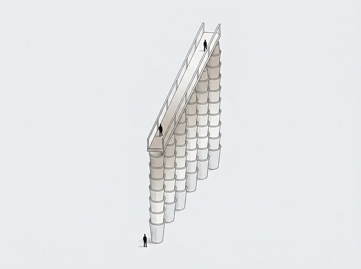
Mapping Latent Operational Volume
Unspent potential sits on the negative side of the enterprise baseline. Every enterprise retains unspent operational potential embedded within inefficient coordination structures and under-automated administrative workflows. Reclaiming this potential demands restructuring internal operating models before committing new financial capital.
Capital committed to a well-structured operating model exhibits high absorption velocity and predictable return gradients.
Friction points within enterprise operations highlight exact coordinates where existing models fail to absorb new capital. An engineering team unable to ship software updates, a sales pipeline stalled by contract governance, or a supply chain constrained by manual warehouse sorting each mark exact boundary walls. Treating these coordinates as structural signals prevents enterprise leaders from throwing capital at fixed operational limits.
Whether enterprise leadership can identify the exact boundary where incremental capital ceases to build capacity remains an unresolved operational challenge.