
Setting Baselines To Calculate Real Operational Variance
Operational baselines anchor past throughput rates across fixed calendar windows to isolate systemic drift from random environmental variance.
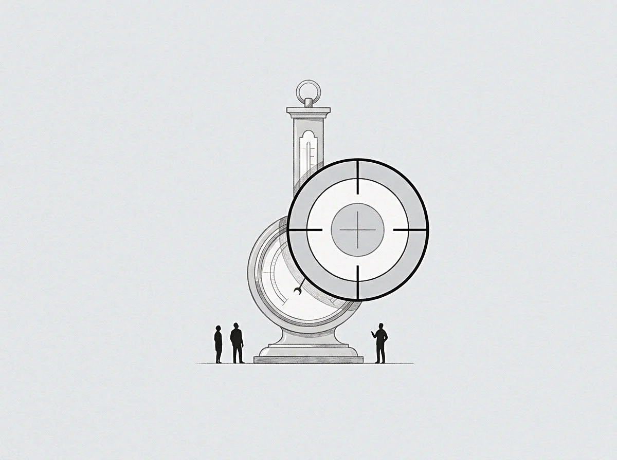
Floor
Production metrics recorded during periods of peak capital injection or temporary team surges create synthetic standards that decay the moment normal operational friction returns. An engineering team operating under the pressure of a delayed release cycle posts completion rates forty percent above sustained capacity for six consecutive weeks. Once delivery concludes, output drops below historical averages as accumulated fatigue extracts its settlement in delayed reviews, deferred refactoring, and absent staff.
When the operator treats that surge velocity as the true performance benchmark, every subsequent month registers as an unexplained shortfall.
A true operational baseline establishes the sustainable rate of output generated when an organization runs without drawing down hidden reserves of goodwill, deferred maintenance, or uncompensated labor. Setting this baseline begins with the identification of unencumbered throughput: the quantity of work completed per unit of time under standard operating conditions. Standard conditions exclude crisis interventions, executive expediting, and temporary resource reallocations.
Establishing this level demands tracking historical output across quiet operational stretches rather than milestone sprints.
A performance baseline calibrated on emergency throughput records routine stability as systemic failure.
The calculation of operational variance isolates structural deviations from expected system behavior. Raw variance combines environmental noise, random statistical oscillation, and genuine operational divergence into an undifferentiated number. Without a stationary reference line, management teams respond to random fluctuations with organizational interventions that introduce new instability into production rhythms.
Field measurements in industrial ergonomics indicate that human operators sustain standard operating performance within a narrow variance band of eight to twelve percent around an established median. Deviations exceeding this threshold signal external interference or upstream resource deficits rather than localized operator error. Setting the operational baseline below this median creates chronic organizational complacency, while anchoring it above this band produces persistent institutional strain.
Variance calculated from an uncalibrated starting point registers noise as signal.

Window

Temporal Sampling Parameters
The duration of the observation period dictates whether an operational metric reflects systemic performance or localized disruption. Short observation cycles capture day-to-day volatility driven by shifting queue lengths, vendor delays, or temporary staffing absences. Long cycles smooth over acute degradations until corrective intervention arrives too late to preserve customer commitments.
Selecting the observation window requires aligning measurement intervals with the natural cycle time of the underlying workflow. A high-frequency customer onboarding workflow completing fifty units daily yields a reliable baseline across a trailing thirty-day window. An enterprise delivery process with an average fulfillment cycle of ninety days demands a rolling four-quarter baseline to account for contract seasonality and client validation cadences.
Shortening this evaluation period produces false variance readings driven entirely by incomplete workflow stages.
The table below contrasts standard baseline configurations across primary operational functions, demonstrating how cycle duration dictates variance thresholds and corrective triggers.
| Workflow Category | Baseline Window Duration | Measurement Metric | Expected Variance Band | Intervention Setpoint |
|---|---|---|---|---|
| High-Volume Transaction Processing | 30 Calendar Days | Settled Units Per Station Hour | Plus or minus 5.0 percent | Two consecutive shifts outside band |
| Mid-Cycle Enterprise Integration | 90 Calendar Days | Milestone Completion Ratio | Plus or minus 11.5 percent | Single milestone delay past ten days |
| Long-Cycle Capital Deployment | 365 Calendar Days | Asset Commissioning Velocity | Plus or minus 18.0 percent | Cumulative quarter deviation past eight percent |

Filtering Seasonal and Exogenous Shocks
External disruptions distort baseline validity if left unadjusted in the primary dataset. A logistics network running during an extreme winter weather event experiences delivery latency three standard deviations beyond normal operational parameters. Incorporating these raw event records into the running baseline inflates variance tolerance across all subsequent periods, masking internal delivery degradation.
Isolating exogenous shocks requires applying fixed exclusion criteria prior to variance computation. Unplanned system outages caused by third-party infrastructure providers, regulatory trade embargoes, and extreme weather interruptions qualify for mathematical quarantine. Quarantined intervals maintain their operational logs for continuity analysis while their throughput figures drop out of baseline rolling averages.
Isolating exogenous shocks preserves baseline sensitivity by preventing transient external disruptions from distorting sustained operating boundaries.
Unfiltered external events corrupt the baseline calculation permanently. The system absorbs environmental volatility into its institutional norms. Operational drift then passes unnoticed.
A written exclusion covenant defining specific environmental anomalies preserves baseline integrity by removing external shocks from the moving average calculation.
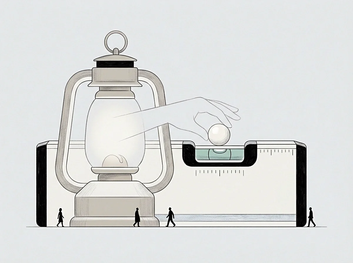
Friction

Endogenous Resistance Mechanisms
Every operational system accumulates internal resistance as transaction volume expands. Structural drag increases through layered approval hierarchies, fragmented communication handoffs, and software dependency tangles. Left unmonitored, internal friction consumes productive bandwidth, shifting the operating baseline downward over successive quarters.
Tracking internal drag requires measuring process cycle efficiency, defined as the ratio of value-adding time to total lead time. In software engineering organizations, developers allocate productive hours across new product logic, maintenance work, and administrative reporting. As organizational architecture expands, coordination overhead expands nonlinearly.
Tasks once executed within hours stretch across weeks as handoffs multiply.
The operator who fails to measure coordination drag attributes declining throughput to personal negligence or diminishing employee dedication. The actual mechanism sits in systemic impedance. Communication lines multiply quadratically with team headcount growth, converting available operational hours into administrative synchronization sessions.
- Coordination overhead consumes operational capacity when inter-team dependencies multiply without shared synchronization protocols.
- Architectural debt diverts developer velocity into manual defect patches and regression monitoring.
- Approval staging delays execution momentum while projects sit idle awaiting multi-stakeholder consensus.

Calculating Real Operational Variance
Distinguishing authentic operational variance from baseline drift demands a multi-factor calculation that strips systemic friction from gross throughput figures. Gross variance represents the raw arithmetic delta between actual output and baseline expectations. Real operational variance isolates the unabsorbed component of that delta after subtracting known coordination overhead and seasonal demand shifts.
Take an operational unit with an established baseline throughput of one thousand service tickets per month. In the fourth month, completed tickets fall to eight hundred. Gross operational variance registers as a negative twenty percent deviation.
Closer structural examination shows three veteran team members spent forty collective hours training eight new hires, absorbing one hundred and twenty tickets of productive capacity. Technical debt caused sixty hours of unbudgeted system downtime, accounting for another fifty tickets.
Adjusting for these quantifiable internal frictions leaves a residual negative variance of thirty tickets, or three percent. This three-percent variance sits comfortably within the natural ten-percent operating tolerance band. Management panic over a twenty-percent collapse reflects mathematical failure rather than execution breakdown.
A gross variance calculation measures systemic symptoms while adjusted real variance isolates actionable operational failure.
Execution stalls when structural friction hides behind raw output numbers. The machine grinds slowly. The team absorbs the cost.
The team completed every assigned task on schedule despite the software failing twice this week.

Coordinate

Mapping the Operational Floor
An operational system reveals its structural limitations at its lowest sustained production boundary. The operational floor represents the minimal viable throughput an organization generates under severe constraint before systemic decay becomes irreversible. Tracking this coordinate provides the reference baseline necessary to evaluate high-stress performance degradation.
When unexpected disruptions reduce available operational resources, managers make immediate decisions regarding workflow preservation. Some workflows must continue uninterrupted to preserve company viability; others accept deferral without inflicting long-term institutional damage. The operational floor maps precisely which activities remain non-negotiable under duress.
Determining this boundary prevents unmeasured organizational collapse during market contractions or acute capital drawdowns. Systems that lack a defined floor attempt to maintain identical performance commitments across all production lines simultaneously. The consequence is generalized quality decay across every business unit.
The operational limit sits at the edge of current capability. Reaching it generates severe administrative discomfort. This friction represents pure computation rather than failure.
Whether human capacity can sustain constant baseline calibration without institutional cynicism remains an open question for operators designing long-term monitoring systems.