
Liquidity Allocation Mechanics during Fixed Capacity Inflection Points
Liquidity allocation during fixed capacity inflections requires pre-funding step-cost outlays while isolating working capital buffers from operational friction.

Choke
A manufacturing plant operates at ninety-four percent of physical throughput when the second assembly line halts for scheduled retrofitting. Daily cash generation drops forty percent within thirty-six hours, while accounts payable for raw material orders placed six weeks prior fall due simultaneously. Capital committed to the expansion project sits locked in transit as unpaid hardware invoices, leaving the treasury depleted before the new line processes a single unit.
Operating at the boundary of physical infrastructure transforms smooth financial projections into steep step-function exposures.
Fixed capacity inflection points occur when an operational asset reaches a physical, technical, or regulatory ceiling where incremental expansion demands a discontinuous outlay of liquid reserves. Linear financial models assume smooth scaling, where incremental revenue matches incremental outlay. Physical systems behave differently.
Pushing past an established operational ceiling demands lump-sum capital commitments long before the asset produces additional cash flow. During this build phase, operational costs per unit rise due to overtime pay, equipment wear, and thermal or computational throttling. The marginal cost curve turns upward sharply while revenue stalls against the ceiling.
Treasury management during this transition relies on mapping the cash depletion rate against the asset installation timeline. Liquid resources flow out along two distinct vectors: baseline maintenance of existing operations and pre-funding of structural additions. When an organization runs close to its operational limit, friction absorbs additional cash.
Orders backlog, customer support queues lengthen, and working capital requirements expand because inventory spends longer waiting for processing slots. This accumulation of unprocessed material locks capital in physical form, preventing conversion back into liquid form.
Miscalculating the timing of this operational junction drains cash reserves faster than non-linear capital expenditure schedules predict. Financial projections that treat plant capacity as a continuous variable fail to account for the cash baseline required to keep old hardware running while new hardware remains offline. Operating past optimal infrastructure parameters generates hidden expenses that strip the balance sheet of flexibility right when expansion payments become mandatory.
Bench
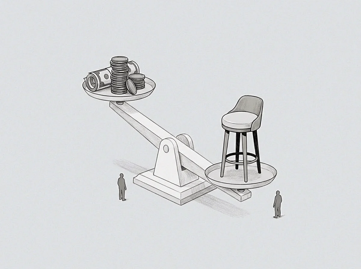
Strategic reserve management requires segregating liquid buffers into distinct functional buckets before capacity limits are reached. Liquidity sitting on the balance sheet often appears fungible, yet cash assigned to cover step-cost outlays cannot simultaneously support working capital spikes caused by process bottlenecks.
Take an organization running two primary operational divisions with a combined annual revenue of fifty million currency units. The enterprise operates a centralized processing core currently running at ninety-eight percent of maximum technical capability. Upgrading this structural core costs twelve million units, payable in three milestone installments across a nine-month construction window.
During this build window, the cash conversion cycle lengthens from forty-five days to eighty-two days as hardware integration creates temporary operational delays. If the firm maintains a flat liquidity baseline of five million units without earmarked allocation tiers, the simultaneous arrival of the second construction milestone and a seasonal spike in inventory inventory absorption completely exhausts available cash.
Fixed capital commitments executed at full capacity collapse liquid buffers unless working capital expansion is pre-funded separately.
Systemic liquidity allocation under capacity constraints relies on three formal structural mechanisms:
- Working Capital Absorption Buffer isolates cash assigned strictly to absorb operational delays, lengthening inventory cycle times, and delayed receivables during construction windows.
- Step Cost Pre Funding Directives lock milestone capital payments into segregated high-liquidity instruments that mature on precise vendor payment dates, keeping them outside operating expenditures.
- Capacity Rationing Surcharge Mechanics adjust internal transfer pricing to temper demand from sales units, intentionally slowing volume growth until the infrastructure addition completes.
Contractual terms with key vendors set the exact boundary of liquidity exposure during these build cycles. A clause specifying payment upon physical delivery rather than payment upon operational commissioning shifts the liquidity risk directly onto the purchasing balance sheet. Negotiating milestone releases contingent on verified throughput thresholds protects treasury reserves against asset integration stalls.
Gradient
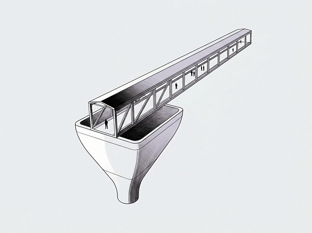
Visualizing liquidity depletion against infrastructure expansion requires plotting a capital expenditure gradient. The axis measures total output relative to maximum fixed capacity. The gradient represents the instantaneous change in liquid capital needed to generate one additional unit of operational throughput.
Below eighty percent capacity, this gradient sits near zero; expansion costs scale linearly with volume. As operational utilization approaches one hundred percent, the gradient steepens sharply. Every marginal increment of output requires exponentially higher cash support to overcome physical friction, thermal limits, or operational overtime.
The optimal liquidity allocation strategy matches the underlying state of asset utilization. The table below delineates the operational behavior, liquidity velocity, and structural risk across distinct capacity regimes.
| Capacity Regime | Operational Behavior | Liquidity Velocity | Capital Intensity Vector | Operational Leverage Risk |
|---|---|---|---|---|
| Linear Scaling Band | Below 80% maximum capacity. Standard throughput. Predictable maintenance cycles. | Low and steady. Cash conversion timing aligns with standard working capital terms. | Minimal. Marginal cost remains constant across incremental volume steps. | Low. Internal cash generation easily covers variable operating outlays. |
| Transition Plateau | 80% to 100% capacity. Extreme asset utilization. Escalating process friction. | Accelerating. Cash tied up in rising inventory backlogs and maintenance spikes. | Steepening. Marginal output costs increase due to inefficiencies and overtime. | High. Margin compression coincides with mandatory lump-sum expansion spending. |
| Post Inflection Expansion | Step-capacity added. Initial underutilization of new hardware core. | High initially, then decelerating as new asset volume absorbs fixed overhead. | Step-function drop in marginal production cost once operational. | Moderate. Revenue must scale quickly to absorb newly elevated fixed asset cost. |
Why do capital buffers exhaust before capacity expands?
Buffer depletion occurs because operating near maximum capacity causes friction that consumes cash faster than financial models anticipate. Machinery operating continuously without maintenance windows breaks down more frequently. Software servers pushed past bandwidth limits incur high latency costs and emergency compute surcharges.
Staff working prolonged overtime earn higher wage rates while productivity per hour declines. The system consumes higher liquid resources simply to maintain its existing output level, leaving zero cash margin to fund the physical expansion required to resolve the bottleneck.
Operational friction at capacity limits converts liquid assets into unproductive overhead before expansion project spending begins.
Creditors analyzing the enterprise during this inflection point view the sudden drop in liquidity velocity as an indicator of operational distress rather than a planned investment sequence. Debt covenants tied to working capital ratios or fixed-charge coverage ratios trigger defaults if liquidity falls below contractual baselines during the integration phase. Lenders demand higher interest margins or tighter covenants precisely when the enterprise needs flexible capital access, increasing the overall cost of capital right at the inflection point.
The counterparty reviewing the financial statements sees an enterprise burning cash at twice its historical rate without an immediate increase in top-line revenue, and demands immediate capital preservation measures before approving further credit drawdown.

Yield
Once new physical capacity achieves operational readiness, liquidity allocation shifts from capital preservation to yield recovery. Commissioning new hardware or facilities resets the marginal operational cost curve downward, but liquidity recovery contains an inherent operational lag. Revenue generation does not step up instantaneously to match newly created infrastructure volume.
Restoring balance sheet liquidity following a capacity inflection follows a predictable, non-negotiable operational sequence:
- System Calibration Phase verifies that newly installed fixed capacity meets operational throughput targets without triggering unexpected fault conditions or elevated waste rates.
- Volume Ramp Execution releases queued order backlogs into the expanded processing environment, translating accumulated raw inventory into completed deliverables.
- Working Capital Normalization reduces safety stock requirements as processing times settle back to design baselines, freeing cash previously tied up in pipeline inventory.
- Treasury Reserve Replenishment directs incoming operational cash flows directly into liquid cash equivalents, restoring liquidity buffers before committing to secondary capital projects.
Balance sheet recovery relies on prioritizing reserve replenishment over premature capital distributions following operational commissioning.
Managing the yield recovery phase requires treating liquidity restoration as a closed control loop. The setpoint represents the target cash reserve level required to sustain business operations at the new baseline. The error signal measures the gap between actual liquid reserves and this target setpoint.
When the error signal remains positive, management directs operational cash flow strictly to treasury reserves. Allocating cash to new growth initiatives while the balance sheet buffer remains below target exposes the enterprise to severe insolvency risk if secondary demand fluctuations occur.
Liquid capital moves toward the path of least resistance when operational limits relax.

Bound
Every operational architecture contains a structural boundary wall. This wall consists of the actions, investments, and operational changes an enterprise refuses to execute because the financial or organizational cost appears prohibitive. Pushing against this boundary generates operational discomfort, which serves as a direct computational measurement of systemic friction rather than a managerial failure.
Avoidance of this boundary creates unprocessed operational debt, which manifests as structural inefficiency, fragile supply chains, and inadequate liquidity reserves.
Mirroring the negative gradient of liquidity depletion reveals the latent potential resting above the baseline. The exact volume of cash consumed by operational friction at ninety-nine percent capacity represents the magnitude of liquid reserve unlocked once the system operates within its design parameters again. Operating at the boundary forces decision-makers to compile a realistic mental model of system limits based entirely on operational failures.
An unexpected hardware failure during a high-volume run identifies the precise technical coordinate of the model boundary.
Friction measured at the capacity ceiling defines the upper bound of current operational architecture.
Discomfort experienced during a capacity inflection measures the computational energy required to transform the operating model. An enterprise that respects its physical walls allocates liquidity to expand those walls before infrastructure friction drains treasury reserves. The boundary marks the precise coordinate where old allocation mechanics cease to function, demanding a structural shift in how liquid capital supports physical capability.