
Calculating Directional Gradient Vectors From Normalized Baseline Performance Metrics
Directional gradient vectors calculate system trajectory and friction by computing partial derivatives across normalized baseline performance metrics.

Desk
Standard dashboards track absolute altitude across time, whereas directional gradient vectors calculate velocity and slope relative to an established operating baseline. Raw metrics present a snapshot of historical accumulation. A scalar output figure of ten million dollars, or a user retention count of eighty percent, reveals where a system sits at a single moment.
It discloses nothing about the force required to keep the system at that coordinate, nor does it indicate whether the underlying trajectory is ascending, plateauing, or decaying into a descent corridor.

Baseline Metrics versus Directional Vectors
Tracking scalar output numbers creates a static portrait of performance that masks underlying system momentum. When a performance metric is evaluated without computing its directional gradient, management decisions respond to past acceleration rather than present inclination. Calculating directional gradient vectors from normalized baseline performance metrics replaces static positional reporting with dynamic force vector analysis.
The calculation requires two distinct steps. First, raw performance metrics across disparate operational domains must be converted into normalized baseline values, stripping out scale differences and establishing a uniform zero line. Second, partial derivatives of these normalized values are calculated across critical operational axes, typically value generated against resources expended.
The resulting vector provides both magnitude and direction, defining the instantaneous path of least resistance within the current operational model. The slope indicates precisely where the system is headed if current inputs remain unaltered.
A gradient computed across normalized baseline metrics isolates directional velocity whenever operational inputs shift faster than output outputs respond.

The Positional Fallacy in Raw Performance Standardizing
A high absolute score often reflects past capital accumulation rather than current operational efficiency. Consider two software deployment units operating within the same firm. Unit A reports ninety-five percent deployment uptime with fifty engineering hours spent per release cycle.
Unit B reports eighty-eight percent uptime with six engineering hours per release cycle. Evaluated strictly on raw reliability, Unit A appears superior. Once normalized against operational expenditure baselines, Unit A exhibits a negative directional gradient vector on the efficiency axis, indicating rising marginal cost per unit of stability.
Unit B exhibits a steep positive gradient vector, demonstrating expanding operational leverage.
Without normalized vector analysis, capital allocation repeatedly flows toward stagnant high-altitude units while starving high-gradient units that are actively compounding efficiency gains above their baseline. When directional vectors consistently point toward paths of lower resistance, structural realignment yields higher efficiency than pushing against accumulated operational friction.

Zero
Establishing a normalized reference line requires converting raw system metrics into stationary statistical distributions across identical observation windows. Baseline performance metrics arrive in heterogeneous units: dollars of margin, milliseconds of latency, customer churn percentages, or support ticket volumes. Direct comparison across these dimensions is mathematically invalid without normalization.
Mathematical Transformations for Baseline Metric Alignment
Converting raw time-series data into standardized statistical distributions removes scale distortion between different operational units. Z-score normalization transforms raw metric values into distance measurements expressed in standard deviations from the historical mean. Min-max scaling compresses raw metrics into a fixed zero-to-one interval based on observed historical bounds.
Rolling median deviation measures performance relative to moving operational medians, dampening the influence of transient operational spikes.
| Normalization Method | Mathematical Formulation | Sensitivity to Outliers | Optimal Operational Context |
|---|---|---|---|
| Z-Score Standardisation | Standard deviation units from window mean | High sensitivity to extreme events | Stationary process metrics with Gaussian distribution profiles |
| Min-Max Scaling | Bounded zero-to-one interval mapping | Moderate sensitivity to bound shifts | Bounded operational limits such as capacity utilization rates |
| Rolling Median Deviation | Absolute deviation from rolling median | Low sensitivity to transient spikes | Volatile environments with frequent non-systemic anomalies |
Selecting the appropriate normalization model ensures that calculated gradient vectors reflect genuine operational shifts rather than statistical artifacts caused by arbitrary scaling choices. Reference-class forecasting in metric variance analysis rests on empirical evaluations of engineering timeline estimates across industrial sectors. This finding holds under stationary mean-reverting environments, though non-stationary operational contexts exhibiting heavy-tailed jump diffusions would invalidate these error bounds.

Structural Comparison of Baseline Normalization Methods
Selecting an appropriate reference standard determines whether calculated slopes reflect true directional motion or statistical noise. When baseline normalization uses an unstable historical window, the resulting zero line shifts continuously, injecting phantom gradient vectors into the analysis. A ten percent change in support ticket resolution speed appears as a major performance surge if calculated against a chaotic baseline window, but shrinks to negligible noise when evaluated against a sixty-day rolling median.
Proper baseline construction locks the reference window length to the natural operational cycle of the unit under evaluation. Quarterly revenue cycles demand longer normalization windows than daily server response metrics. Once normalized values align along a stable zero axis, any deviation from the zero line represents meaningful operational displacement capable of supporting vector calculations.
Misassembling the baseline transforms gradient calculations into random statistical noise, leading operators to deploy capital against fictitious system signals.

Notch
Once metrics are centered around a steady reference point, computing directional vectors involves taking partial derivatives across chosen operational dimensions. Value created sits on the primary vertical axis. Resource expenditure, measured in hours, capital, or attention, sits on the horizontal axis.
The directional gradient vector points in the direction of steepest value growth per unit of resource consumed.

Deriving Vector Components Across Operational Axes
Value creation and resource expenditure form the primary two-dimensional coordinate system for slope calculation. The gradient vector is derived by calculating the rate of change of the normalized performance metric with respect to each operational coordinate axis. In a two-variable system where performance output depends on capital input and engineering labor input, the directional vector consists of two orthogonal partial derivative components.
- Orthogonal Vector Blindness occurs when an operator evaluates performance along a single resource axis while ignoring parallel resource draw, mistaking simple resource shifting for true efficiency ascent.
- Baseline Drift Suppression happens when changing market background conditions elevate raw output metrics, causing operators to calculate positive vectors from environmental tailwinds rather than internal operational improvements.
- Magnitude Distortion From Unscaled Axes emerges when unnormalized resource inputs corrupt the vector angle, skewing the calculated path of steepest ascent toward the largest numerical scale.
The field remains divided on whether persistent avoidance of a specific channel indicates structural friction or accurate intuitive refusal by the operator. Under this analytical uncertainty, the operator runs a low-volume test on the avoided coordinate for two observation cycles to gather empirical rate data before committing structural capital.
Systematic Misreadings in Multi-Dimensional Gradient Estimation
System operators frequently confuse steep scalar ascents with sustainable operational trajectory. A rapid increase in top-line output often masks an equally rapid acceleration in resource consumption. When the partial derivative of output with respect to capital equals the marginal cost of capital, further movement along that vector yields zero net value accumulation.
Evaluating directional gradient vectors requires isolating the magnitude of the vector from its angle. A high-magnitude vector pointing steeply toward the cost axis indicates that the system is burning capital at an unsustainable rate to achieve marginal performance gains. Conversely, a moderate-magnitude vector aligned closely with the value axis demonstrates high structural leverage.
The output was supposed to match the projection because the baseline figure showed continuous growth throughout the previous quarter.

Plane
Plotting gradient vectors onto an operational surface reveals where the system naturally drifts along the path of least resistance. Descent represents the natural trajectory of any unconstrained system. Systems naturally move down energy slopes, avoiding complex administrative or technical tasks that impose heavy immediate computational costs on operators.

Why do system boundaries concentrate unprocessed material?
Systems naturally route energy around high-cost operational tasks, accumulating administrative backlog at the exact edge of current technical capability. What an organization systematically routes around reveals where unprocessed material builds up behind operational barriers. That accumulated volume mirrors the exact magnitude of latent potential sitting unused above the baseline.
Research on cognitive load asymmetry between approach and avoidance choices rests on controlled laboratory trials measuring task-switching latency in multi-objective decision loops. The conclusions apply directly to human operational environments, though high-frequency automated decision systems with real-time feedback loops eliminate these cognitive latency disparities. Naval navigators calculate current drift vectors relative to true heading rather than relying on visible shorelines.
That same vector mathematics applies when isolating operational momentum from background market movements.
- Measure raw performance indicators across a fixed ninety-day window.
- Normalize scores using zero-mean unit-variance transformation across all units.
- Compute partial derivatives along value and effort dimensions simultaneously.
- Invert the negative gradient vector to map unspent latent volume.
- Align operational resources with the calculated ascent trajectory.
A system routing work around a high-cost node reveals the true boundary of its current operational model.
Sequential Derivation of Mirrored Latent Potential
Mirroring the descent gradient vector directly above the normalized baseline flips the trajectory from least resistance to latent opportunity. The descent vector identifies where the organization routinely surrenders efficiency to avoid friction. Flipping this vector along the baseline axis yields the precise directional vector required to capture unspent capacity.
The magnitude of the mirrored vector equals the magnitude of the avoidance vector. If a product engineering group consistently avoids refactoring legacy core architecture, routing all feature work through external API wrappers, the negative gradient along the codebase maintenance axis is steep. Reversing that coordinate reveals the unspent potential available if structural refactoring is completed.
Applying the latent potential inversion clause changes the operational allocation by redirecting unspent engineering capacity toward the specific bottleneck the model previously bypassed.
Sheath
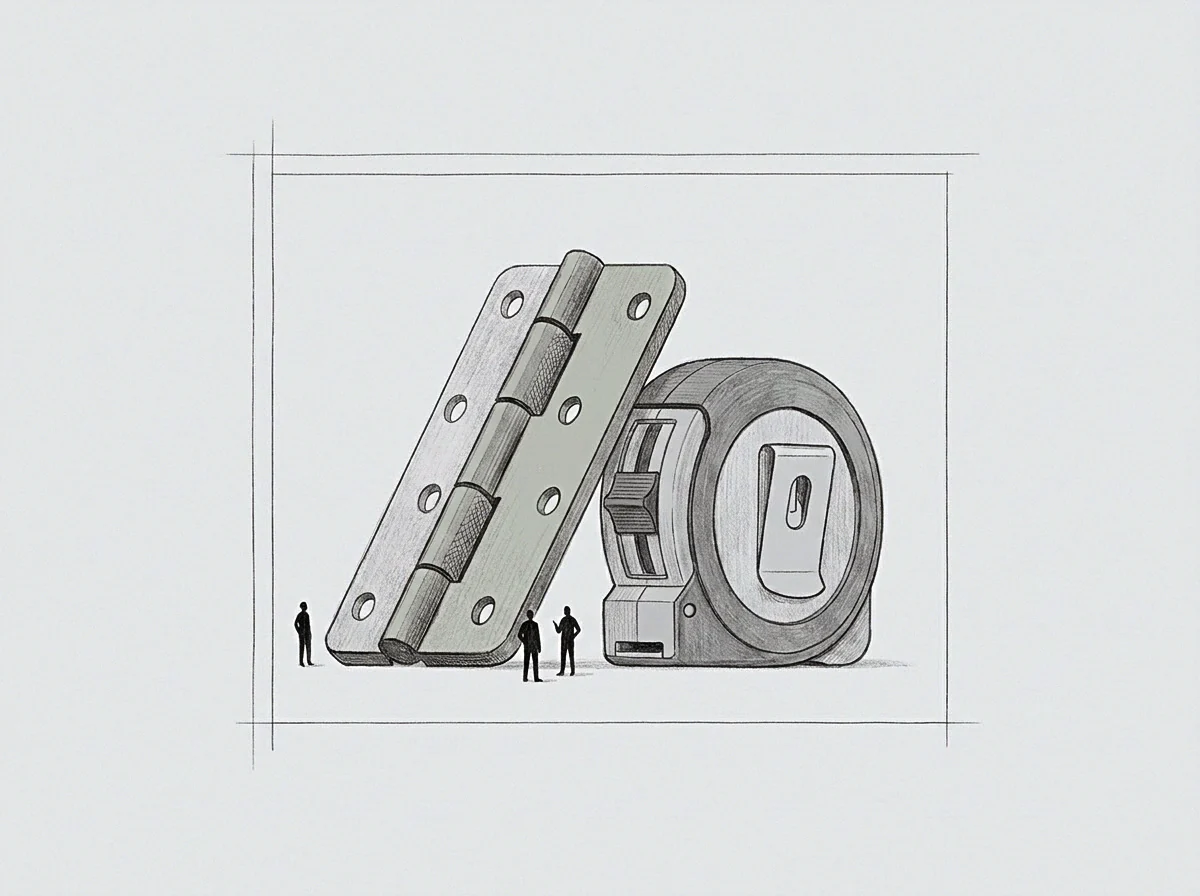
The boundary enclosing a system model consists of the exact set of tasks the organization refuses to perform due to high immediate computational cost. This boundary wall is constructed from what the system routes around. When an organization reaches its boundary wall, every unit of additional output demands exponentially higher resource inputs, resulting in a steep, near-vertical cost gradient vector.
Mapping Model Boundaries Through Operational Discomfort
Internal friction signals active computation rather than operational failure. When an operator encounters severe operational resistance at a specific coordinate, the current model is attempting to process inputs that exceed its algorithmic capacity. System errors compiled at this boundary provide exact numerical coordinates for expanding the model.
A failure is not a loss of vector momentum; it is a point measurement defining the boundary surface. By recording the precise location of system stalls across normalized performance baselines, the operator constructs a complete map of the current operational container. Expansion occurs exclusively by pressing directly against these recorded boundary coordinates.
An operational gradient exceeding forty degrees on the cost axis indicates an imminent system boundary wall.
Gradient vectors calculated from normalized baselines eliminate personal narrative from operational evaluation. The vectors report directions, magnitudes, and boundary positions with absolute mathematical neutrality. Whether an organization can systematically alter its boundary wall without first experiencing complete operational stall on its primary value axis remains an open empirical question.