
Computing Directional Gradient Vectors From Value Variance Beyond Two Dimensional Quadrants
Computing directional gradient vectors derives continuous rates of value variance across multi-dimensional surfaces to guide movement beyond flat quadrants.

Surface
Operational reality rarely sits neatly inside two axes. Evaluation systems frequently attempt to compress decisions into four-box matrices, forcing complex inputs into orthogonal pairs such as effort against impact or urgency against importance. When a project carries variance across latent dimensions including attention, technical liquidity, regulatory risk, and team energy, flat models break down.
Value forms a continuous landscape. Compressing multi-variable operational space into flat grids hides the true direction of maximum progress.
Calculating gradient vectors requires treating value as a continuous scalar field distributed over multi-dimensional inputs. The gradient vector points in the direction of steepest value increase, with its magnitude describing the local rate of change. When variance shifts along unrecognized dimensions, calculating partial derivatives along each active axis reveals actual slope rather than projected priority.
The gradient tracks maximum rate. A team evaluating initiatives along five distinct variance axes discovers that the path of optimal return rarely aligns with any single axis in isolation.
When variance spans multiple operational axes, calculating partial derivatives along each coordinate identifies the vector of maximum output growth.
Static evaluation frameworks treat coordinates as fixed points within quadrants. Real operational environments exhibit continuous drift across all parameters simultaneously. Variance across axes alters slope.
Evaluating a system through static positions produces misallocated capital because the underlying surface changes while the coordinate markers remain stationary. A project positioned in a high-impact quadrant can simultaneously experience severe gradient descent toward baseline loss if secondary dimensions experience unmonitored decay.
Failing to compute multi-dimensional gradient vectors forces decision structures to rely on arbitrary quadrant boundaries, causing capital allocation to track historic categories rather than active rates of value creation.
Wall

Operational Boundaries and Resistance
The boundary of an operational model defines what the structure refuses to compute. In multi-dimensional space, system boundaries manifest as steep gradients of rising ordinal cost, representing zones where minor operational shifts demand exponential energy. Discomfort marks active computation at these limits.
Vectors reveal hidden drag. When an initiative approaches an operational constraint, the value variance flattens, indicating that further progress along that trajectory requires structural modification rather than simple resource injection.
Assume an organization evaluates product expansion across four continuous variance axes: engineering bandwidth, customer acquisition cost, compliance overhead, and brand equity. Traditional two-dimensional quadrant mapping places the project in an favorable category based solely on acquisition cost and market size. Incorporating compliance overhead and engineering bandwidth into the gradient calculation alters the vector direction by ninety degrees.
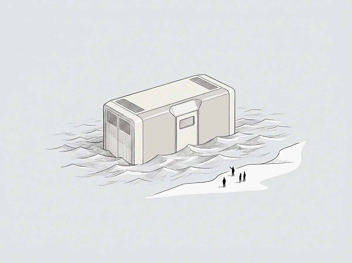
The updated vector demonstrates that moving forward without addressing technical debt drives the system directly into a wall of execution friction.
- Quadrant Compression occurs when multi-dimensional variance is forced into two axes, masking critical drag factors that alter true trajectory.
- Boundary Reflection happens when a system meets an unmodeled limit, bouncing operational effort into unproductive side projects without advancing core metrics.
- Static Trajectory arises from treating directional vectors as permanent paths rather than continuous derivatives subject to real-time recalculation.

Internal System Thresholds
System friction accumulates where unprocessed variance sits unmonitored. Static grids miss directional velocity. When an operational team routes work around a specific technical or organizational constraint, that avoidance behavior marks the exact coordinates of an unmapped barrier.
Measuring the magnitude of avoidance provides the exact dimensions of the obstacle sitting behind it.
Unaddressed operational friction creates a persistent deflection vector, forcing organizational output away from high-value trajectories.
A system operating under unmapped constraints consistently converges toward local minima. The path of least resistance directs effort downward along the baseline, away from high-yield objectives that demand structural compute. Climbing requires deliberate energy.
The mirror above the baseline displays unspent latent potential equal in magnitude to the energy spent avoiding the wall.
The boundary clause within an operational mandate determines whether a team expands its computational surface or retreats into familiar quadrant boundaries when encountering friction.

Projection

Directional Derivation Across Coordinates
Computing gradient vectors in high-dimensional spaces relies on isolating partial derivatives across every variance axis. The scalar value function assigns an output figure to every combination of input variables. The surface shifts under load.
Differentiating this function with respect to individual parameters yields a directional vector that quantifies rate of change across the entire surface.
- Identify every active axis contributing to output variance across the operating unit.
- Compute partial derivatives across continuous scalar inputs to isolate individual variable rates.
- Construct the partial vector array to map maximum ascent across the multi-dimensional surface.
- Compare the directional vector against operational capacity to ensure execution feasibility.
Which Matrix Identifies Directional Shift?
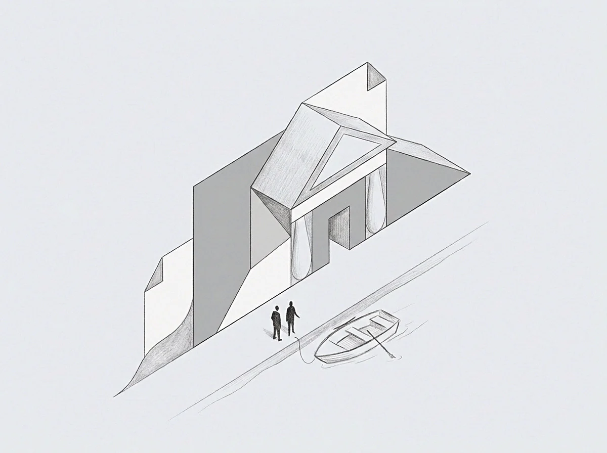
Mathematical projection onto lower-dimensional sub-spaces permits visualization without losing vector integrity. Local minima trap unspent capacity. Projecting a five-dimensional gradient vector onto a reduced operational plane reveals how secondary variables distort primary goals.
The variance-covariance matrix exposes hidden dependencies between inputs, showing where two seemingly independent parameters move in tandem to resist operational shifts.
Measurement precedes effective movement. When internal dependencies remain hidden, attempts to push an initiative along a positive value vector produce unexpected drag along unmonitored coordinates. The boundary marks local resistance.
Tracking the directional derivative along the full variance array ensures that movement aligns with actual surface topology rather than idealized projections.
The engineering lead noted that the proposed expansion trajectory looked optimal on the slide deck but collided directly with unmodeled database scaling limits.

Asymmetry
Ordinal Cost Versus Cardinal Price
Cardinal price captures discrete monetary transaction figures. Variance expands existing models. Ordinal cost reflects the relative draw on structural energy, cognitive bandwidth, and option liquidity required to execute a directional shift.
Directional vectors guide structural shift. Two initiatives carrying identical financial budgets frequently exhibit vastly different ordinal costs based on where they sit relative to the current operational model boundary.
| Evaluation Criteria | Two-Dimensional Quadrants | Directional Gradient Vectors |
|---|---|---|
| Input Capacity | Restricted to two orthogonal axes | Accommodates arbitrary continuous dimensions |
| Variance Detection | Categorical grouping inside static boundaries | Continuous derivative measurement across surface |
| Trajectory Mapping | Fixed position assignment without velocity | Directional vector carrying magnitude and orientation |
| Constraint Handling | Ignores unmodeled variables outside two axes | Identifies boundary friction through gradient decay |
Unprocessed load creates system friction. Evaluating strategic direction purely through cardinal pricing metrics creates structural asymmetry. An initiative requiring modest financial outlay can exhaust organizational capacity if its vector runs perpendicular to existing operational pathways.
Conversely, significant capital deployment along the natural ascent gradient moves smoothly because internal structures already support that trajectory.
Directional clarity emerges from calculating vector slopes rather than assigning arbitrary category labels inside static grids.
Each axis carries distinct weight. Ordinal scale ranks resource draw. Strategic alignment improves when decision models incorporate the relative ordinal cost of shifting directions alongside cardinal price projections.
Systems follow the path of least resistance unless explicit directional force overrides internal inertia.
Contour

Latent Potential Beyond Local Minima
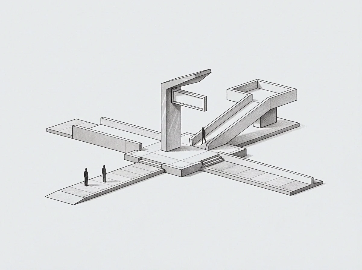
Mapping contours across multi-variable surfaces highlights regions of latent potential that flat quadrant analysis obscures. A contour line connects points of equal value across the landscape. When contours sit densely packed, minor operational adjustments yield substantial changes in overall output.
Broadly spaced contours indicate flat regions where additional effort produces negligible return.
Persistent avoidance of specific operational tasks marks the precise coordinate of unspent latent potential.
Navigating out of local minima requires moving against immediate slope descent. The path of least resistance pulls systems down into comfortable operational valleys where value creation stalls. Climbing demands deliberate, energy-intensive vector movement upward toward higher contours.
Reaching peak potential demands traversing areas of elevated operational discomfort where internal models expand to absorb new complexity.
Directional gradient vectors provide objective measurements of trajectory without introducing subjective scorekeeping. The mathematical derivative reports slope, magnitude, and boundary friction as raw structural facts. Operators applying continuous multi-dimensional gradients locate high-yield ascent vectors while maintaining operational clarity across changing environment conditions.