
Mapping Multivariable Process Variance Manifolds To Calculate Value Trajectories
Multivariable process variance manifolds map operational fluctuations across state space to project scalar value trajectories along local rate vectors.
Slope
An enterprise logistics system monitoring forty distinct operational parameters maintains tight statistical control across every individual variable, yet net economic yields decline by twelve percent over consecutive quarters. Standard diagnostic tools examine univariate distributions, treating each metric as an isolated process channel. This approach misses the geometric reality of complex operations.
When multiple process inputs oscillate simultaneously, their combined fluctuations trace out a continuous high-dimensional surface rather than a collection of independent lines. The geometric curvature of this multivariable surface dictates how performance evolves over time.
State Space Geometry and Covariance Structure
Operations unfold within a high-dimensional state space where every process metric defines a coordinate axis. Parameter variations form an empirical covariance structure that reflects true systemic interaction. When two operational parameters move together, their shared variance distorts the surrounding performance field.
Measuring univariate variance alone paints a misleading picture of systemic stability. A process may report low variance on every single metric while the combined state vector wanders into regions of severe inefficiency.
The baseline configuration of an operational process establishes a reference point in this state space. Eigenvalue decomposition of the empirical covariance matrix isolates the principal axes of variance. These axes define the orientation of the variance manifold.
The magnitude of each eigenvalue reveals how much operational instability accumulates along that specific geometric direction.
When variance components align along coupled axes, local optimizations flatten the overall scalar output trajectory.
Processes naturally drift along directions defined by large eigenvalues. This movement represents the path of least physical or organizational friction within the system. Operators who ignore the underlying geometric manifold end up wasting effort on parameters that have minimal structural impact on net output.
Multivariable Process Variance as Topological Surface
Visualizing process behavior as a topological manifold transforms continuous operational monitoring into a geometric problem. The manifold bends and folds according to systemic feedback loops and resource constraints. High variance in one operational quadrant often forces compensatory shifts in adjacent parameters, warping the surrounding surface.
This structural warping changes the path that future process states will follow.
Mapping this surface requires calculating local curvature matrices across discrete time windows. Rapid shifts in local curvature indicate impending process transitions or structural bottlenecks. Where the manifold bends sharply, minor operational perturbations trigger significant performance swings.
Tracking these topological features gives engineers early warning before net economic output degrades.
Systemic friction distorts the manifold shape. Execution leaves a trace. When process variance accumulates without intervention, the underlying surface forms steep local wells that trap performance.
Standard optimization routines get stuck in these structural troughs, failing to locate higher efficiency regions situated across steep geometric barriers. The financial consequence of treating a multivariable variance manifold as a collection of independent parameters is the progressive accumulation of unmanaged operational risk across linked execution channels.

Table
Quantifying how operational variance translates into economic trajectory changes requires mapping specific process dimensions against their corresponding topological signatures. Different operational parameters exert unequal influence on the surrounding scalar field. A structured comparison reveals how localized fluctuations destabilize systemic output.
Mapping Operational Vectors Against Value Sensitivity
Operational vectors differ in their structural coupling and resource consumption profiles. The table below evaluates four core process dimensions across key geometric criteria, showing how variance magnitude correlates with trajectory degradation.
| Process Dimension | Variance Topology | Eigenvalue Magnitude | Trajectory Impact | Adjustment Cost Vector |
|---|---|---|---|---|
| Execution Latency | Linear Ridge | High Positive | Immediate Trajectory Decay | Ordinal Schedule Shift |
| Resource Allocation Volatility | Saddle Point | Moderate Bounded | Localized Output Oscillation | Cardinal Capital Reallocation |
| Interface Error Density | Parabolic Well | High Negative | Cumulative Value Atrophy | Structural Redesign Overhead |
| Information Flow Drift | Planar Dispersion | Low Unbounded | Gradual Baseline Erosion | Continuous Governance Drag |
Variance characteristics dictate the stability of the entire operational manifold. High eigenvalue magnitude along negative directions signals rapid performance loss, requiring immediate structural realignment to protect net economic yield.
Systemic evaluation depends on recognizing specific failure modes embedded within the variance topology. Operators use structured diagnostic indicators to categorize the operational surface based on observed variance patterns.
- Linear Ridge Instability develops when execution delays propagate sequentially through downstream process nodes, creating persistent directional drift across the state space.
- Saddle Point Trapping occurs when resource allocation swings wildly between competing process priorities, holding net performance at a sub-optimal equilibrium.
- Parabolic Well Accumulation represents dense clusters of interface errors that attract operational focus and consume capacity without increasing output.
- Planar Dispersion Drift marks subtle, wide-spectrum variances across information workflows that slowly erode baseline efficiency over extended operating periods.
Identifying these structural patterns allows teams to target intervention efforts where geometric sensitivity is highest. Correcting variance along dominant eigenvector directions produces the largest trajectory improvements per unit of effort spent.
Unmapped variance along coupled process axes reduces economic output before individual boundary metrics signal alert.
A process operating under uncalibrated variance limits expands its state footprint until local buffer capacity is exhausted. Stated boundary tolerances establish the operational region where output predictions remain valid, while unmapped variance expansion alters the underlying value equation across all active execution channels.
Wall
Physical limits and contract rules mark the structural boundary of any business process model. When operational states approach these edge conditions, the smooth mathematical relationships defining the manifold break down. Variance vectors that press against hard systemic limits create severe local distortion.
The system can no longer route around operational friction through ordinary parameter adjustments.

Boundary Conditions of the Process Model
Every operational system functions within a bounded domain defined by physical throughput capacity, regulatory parameters, and contractual commitments. As process variance pushes state trajectories toward these outer boundaries, operational flexibility drops to zero. The cost of further variance increases exponentially near the perimeter.
Capital tracks the drift.
Boundary collisions transform continuous variance into immediate operational disruptions. A supply chain operating near maximum warehouse capacity cannot absorb minor delivery timing variations. The excess variance reflects off the boundary wall, destabilizing upstream production schedules and compounding administrative drag.
Mapping the distance between current operating points and fixed boundary walls provides an accurate measurement of systemic resilience. Processes running close to structural boundaries require tight variance suppression routines. Allowing variance to grow near operational limits risks triggering irreversible state shifts that damage long-term asset value.
Discomfort as Computation Signal at the Model Edge
Operational friction and team strain near boundary walls serve as direct measurements of systemic computation. Discomfort signals that the existing operational model lacks the mathematical capacity to process incoming variance within established parameters. The system is working to resolve structural contradictions between process inputs and boundary constraints.
Ignoring these edge signals causes organizations to build artificial workarounds around unmanaged variance hubs. These informal fixes hide true operational costs while expanding the overall complexity of the process manifold. The extra complexity consumes energy without altering the underlying boundary constraints.
Process systems route around unmeasured variance until structural boundaries force explicit computation.
Effective management requires bringing process execution back into regions of the state space where the mathematical model remains fully predictive. Pushing against structural walls yields diminishing returns while accelerating component wear across the organization. The external partner observing these boundary stresses would note that current delivery commitments assume a process stability that the physical operations no longer maintain.
Gradient
Vector calculus provides the mathematical framework for projecting performance changes across high-dimensional variance manifolds. The gradient of the scalar value field points in the direction of steepest output increase, while its negative derivative identifies the path of fastest performance degradation. Calculating these direction vectors allows operators to chart optimal recovery paths across complex state spaces.
Which Variance Vectors Accelerate Value Trajectories?
Determining which process adjustments yield positive trajectory changes requires evaluating the inner product of the local gradient and active variance vectors. Alignment between variance direction and the value gradient accelerates performance growth. Orthogonal or opposing variance vectors degrade efficiency and dissipate operational momentum.
Operators track trajectory changes by executing a systematic step sequence across the operational state space:
- Construct the local empirical covariance matrix from continuous parameter measurements across a specified time window.
- Isolate dominant eigenvectors to identify the primary directional channels of operational variation.
- Compute the local scalar value gradient using partial derivatives of economic yield with respect to each process coordinate.
- Project the active variance vectors onto the value gradient to quantify directional efficiency.
- Adjust parameter constraints along directions that maximize positive gradient projection while suppressing orthogonal noise.
Following this optimization sequence prevents teams from spending resources on variance reduction along axes that do not contribute to net economic performance. Precise vector alignment maximizes the return on operational interventions.

Scalar Value Trajectory Projections
Projecting future performance requires integrating local gradient vectors along expected variance paths over time. Linear extrapolation fails because the manifold surface curves across state space. Accurate forecasting depends on continuous state-space models that update trajectory estimates as process coordinates change.
Variance forces a recalibration. When unexpected operational perturbations shift the process state onto a new section of the manifold, the local value gradient changes orientation. The system must recalculate its forward trajectory to avoid falling into low-efficiency performance basins.
The path of least operational resistance frequently leads toward lower scalar output.
Long-term output trajectories depend on keeping process states aligned with favorable gradient slopes. Operational systems that drift unchecked naturally slide down the value surface into local performance minima. The open analytical challenge remains whether current real-time mapping tools can update high-dimensional process manifolds fast enough to intercept rapid variance spikes before performance drops below baseline recovery thresholds.

Descent
Following the path of least resistance across a process manifold leads downward along the negative value slope. Organizational systems tend to settle into these low-energy configurations because maintaining higher performance positions demands continuous energy input. Reversing performance loss requires deliberate, forced movement against the local variance gradient.
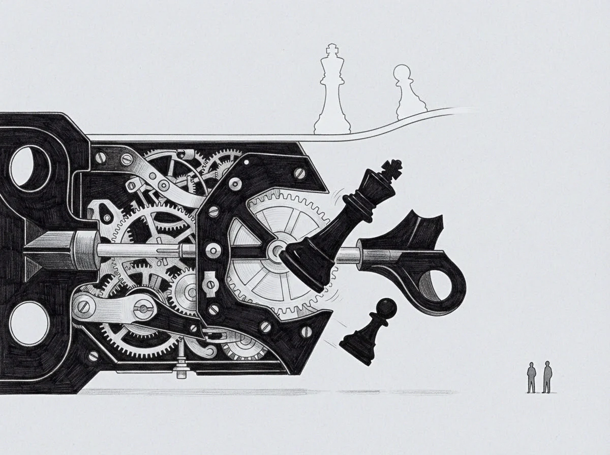
Least Resistance and Latent Potential Recovery
Operational descent occurs quietly as teams adopt workarounds that minimize immediate friction while sacrificing long-term output quality. The vector flips sign. These low-resistance pathways shape the process manifold, creating structural habits that resist passive correction efforts.
Operational friction absorbs the signal.
Mirroring the negative gradient above the baseline reveals the latent potential trapped within unmanaged process variance. This unspent volume represents the performance upside available if the system can eliminate structural inefficiencies and realign process execution with the true value vector. Recovering this volume requires targeted intervention along specific directional coordinate axes.
Cost measures the work. The effort required to elevate a process state out of a performance trough scales directly with the depth of the local manifold basin. Organizations must commit sufficient capital and operational focus to cross high geometric energy barriers into superior operational states.

Projecting Value Trajectories Across State Boundaries
Calculating forward value trajectories requires mapping how state transitions alter systemic capacity over extended operational horizons. As a process moves across different state space regions, changing parameter interactions modify the value landscape. Robust projections account for these geometric shifts rather than assuming static performance conditions.
The trajectory stabilizes. Sustained performance growth occurs when systemic control loops continuously adjust operational inputs to keep the process vector aligned with positive value gradients. Effective governance maintains these directional adjustments despite shifting external inputs and internal process noise.
Mapping multivariable process variance manifolds transforms operational management from reactive troubleshooting into precise geometric navigation. Systems designed with continuous manifold mapping capabilities maintain high performance output across changing operational environments. Unmanaged process variance consistently pulls operations toward the path of least resistance unless active gradient alignment forces continuous performance ascent.