
Reconstructing Latent Variables When System Attractors Suddenly Collapse
Reconstructing latent variables during attractor collapse relies on tracking non-equilibrium energy dissipation rates along structural system boundaries.
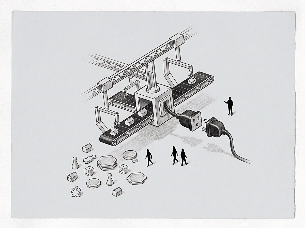
Bifurcation

Dissolution of Phase Space Stability
A telemetry dashboard goes dark when an enterprise routing engine crosses a non-linear threshold, dropping transaction volume from forty thousand requests per second to zero within four minutes. Operational teams view the output drop as a temporary throughput pause, assuming the internal state remains locked near the previous equilibrium setpoint. In complex non-linear dynamics, crossing a saddle-node tipping point destroys the equilibrium basin entirely.
Trajectories migrate rapidly across unstable state spaces toward unmapped boundaries rather than returning to historical normal distribution ranges. Standard estimation routines relying on stationary state assumptions generate invalid readings because the underlying system attractor no longer exists.
The basin dissolves.
Take an operational infrastructure running three microservice layers without stated throughput limits, where latent queuing delays accumulate silently behind database locks. Assume the platform owner observes stable latency metrics right until the primary database connection pool empties. When connection exhaustion strikes, the dynamic baseline vanishes.
Reconstructing internal queuing states through historical observability tools becomes impossible because historical time series metrics reflect attractor dynamics that collapsed during the bifurcation event.
Operational capacity flattens to zero while downstream error logs report nominal throughput during attractor dissolution.
Observability drops to zero.
Latent variables represent hidden internal states, such as internal queue friction, unspent channel capacity, and structural resource debt. When system attractors collapse, these hidden variables dictate whether the platform settles into a dead state or transitions toward an unmapped secondary orbit. Operators who treat zero output as a static idle state miscalculate the internal thermal stress remaining within the service boundary.
The cost of misreading this non-equilibrium state is the immediate destruction of remaining hardware memory buffers when secondary system restarts trigger unmanaged feedback loops.
Floor

Transient Non Equilibrium Tracking
tracking methods designed for steady-state systems fail when internal dynamics accelerate along transient paths. Once the stable setpoint vanishes, state trajectories strike hard operational constraints, such as memory caps, credit limits, or physical queue limits. These physical boundaries act as structural boundaries where energy dissipates through error generation, discarded frames, and unhandled retries.
Measuring latent state vectors during non-equilibrium decay demands tracking dissipation rates directly against these hard physical limits rather than searching for local equilibrium points.
The setpoint disappears.
Energy leaves the system.
Standard manifold reconstruction techniques based on delay coordinate embedding rely on recurring orbits in phase space. When an attractor collapses, trajectories never retrace prior pathways, rendering traditional time-delay state reconstruction mathematically ill-posed. Reconstructing latent parameters under sudden collapse conditions uses non-equilibrium dissipation tracking.
The list highlights failure modes that occur when teams attempt state reconstruction without accounting for attractor dissolution.
- Equilibrium Assumption Mapping treats transient decay trajectories as if the system remains inside a stable historical basin, generating incorrect state estimates.
- Static Gain Observer Application applies fixed Kalman gain matrices during dynamic manifold collapses, causing state estimators to diverge violently from reality.
- Metric Zero Equivalence mistakes the absence of output telemetry for an internal state of zero energy, ignoring latent structural pressure against system walls.
- Linearized Sensitivity Projection projects sensitivity vectors across non-linear tipping points, ignoring higher-order tensor shifts occurring during structural bifurcation.
Noise masks the trajectory.
Latent variable precision improves when measurement sampling aligns with the transient dissipation rate rather than the previous baseline clock.
The coordinate shift holds.
A senior infrastructure partner looking at the zero-output dashboard during an unmapped outage will state that the system is simply waiting for a manual database restart.

Observer
Which Signals Survive Attractor Dissolution?
State estimation during phase collapses requires observers capable of functioning without stationary dynamic models. When system matrices lose positive-definiteness, standard Extended Kalman Filters drift because prediction error covariance matrices grow without bound. Shadow manifold tracking and non-equilibrium energy filtering extract latent variable coordinates by observing cross-variable correlations among surviving peripheral metrics.
Even when primary performance metrics drop to zero, secondary boundary interaction signals maintain measurable correlation structures.
Dissipation accelerates.
Internal friction rises.
Evaluating state reconstruction approaches during structural bifurcation requires comparing observational inputs, latency parameters, and operational failure modes. The table outlines three distinct observer methodologies used to recover unobserved system variables during catastrophic phase transitions.
| Method | Primary Observable | Reconstruction Latency | Failure Boundary |
|---|---|---|---|
| Delay Embedding | Recurrent phase trajectories | Infinite during collapse | Requires stationary attractor manifold |
| Shadow Manifold Tracking | Cross variable correlation vectors | Low during steady state | Fails upon local dimensional expansion |
| Non-Equilibrium Energy Filtering | Dissipation rates along boundary walls | Bounded by sample frequency | Valid while dissipation rate remains measurable |
The baseline resets.
A non-stationary observation matrix causes standard state estimators to interpret transient velocity as continuous measurement noise.
State reconstruction validity hinges on maintaining continuous measurement sampling at frequencies higher than the dynamic collapse rate, a condition that holds only while hardware telemetry channels remain unblocked by primary protocol timeouts.

Gradient

Mapping Unspent Volume Above Baseline
Computing value along system pathways reveals directional slopes without imposing external subjective scores. System trajectories naturally follow paths of least resistance, routing around internal bottlenecks and operational obstacles. When an attractor dissolves, this routing behavior shifts instantly toward peripheral boundary lines.
Mapping where system flows actively avoid operating yields the exact spatial coordinates of latent structural barriers.
The vector flattens.
Transient decay governs velocity.
Mirroring the negative dissipation gradient above the operational baseline reveals the unspent volume of latent system potential. The unspent volume represents processing capacity locked behind structural barriers during non-equilibrium transitions. Executing latent variable reconstruction post-collapse follows a strict sequence of analytical steps.
- Identify surviving peripheral telemetry streams that maintain active measurement signals during main system attractor dissolution.
- Calculate energy dissipation rates along hard hardware and network boundaries to establish non-equilibrium velocity vectors.
- Construct a shadow manifold using cross correlation matrices calculated over moving sub-second observation windows.
- Invert the boundary dissipation vector to compute unspent latent capacity available within the transient system state.
Mirroring the avoidance vector against system boundary walls exposes latent variables hidden by metric zero readings.
The wall limits state recovery.
Static assumptions fail completely.
What structural signal indicates whether an unmapped transient trajectory will settle into a functional secondary attractor or proceed directly toward terminal system shutdown?

Recovery

Restructuring Manifolds After Tipping Points
Reestablishing operational control after attractor collapse requires anchoring reconstructed latent variables to newly synthesized stability basins. Operators cannot force a collapsed system back into its old historical setpoint once the physical phase space topology changes. Attempts to re-impose historical control parameters on a post-bifurcation system trigger severe resonance instabilities.
Reconstructing latent parameters provides the precise spatial coordinates required to construct new setpoints that match the post-collapse topology.
In fluid mechanics and structural mechanics, stress distributions near material failure points undergo sudden spatial realignments when micro-fractures coalesce into main fault lines. Non-linear operational systems mirror this exact behavior, re-routing operational stress vectors along unexpected structural axes during critical tipping events.
Research across non-linear control systems demonstrates that state estimation error bounds expand exponentially when observational model updates lag system phase velocity. Empirical studies in experimental state reconstruction rely on continuous shadow manifold embeddings. These embeddings remain valid provided the intrinsic manifold dimensionality stays below eight, though dimensional expansion during severe thermal or operational stress frequently degrades reconstruction precision.
When dimensional expansion occurs, non-equilibrium energy filtering remains the sole stable estimator, requiring operators to rely entirely on direct boundary dissipation tracking.
Latent state vectors measured along boundary walls during non-equilibrium decay predict post-collapse trajectory targets far more reliably than historical baseline averages.